Research Article | Open Access | 8 Oct 2021

Online monitoring of batch processes combining subspace design of latent variables with support vector data description

Views: 1465 | Downloads: 681 | Cited:

Zhaomin Lv

Complex Eng Syst 2021;1:4.

10.20517/ces.2021.02 | © The Author(s) 2021.

Author Information

Article Notes

Cite This Article

Abstract

The correlation relations of batch process variables are quite complex. For local abnormalities, there is a problem that the variant features are overwhelmed. In addition, batch process variables have obvious non-Gaussian distributions. In response to the above two problems, a new multiple subspace monitoring method called principal component analysis - multiple subspace support vector data description (PCA-MSSVDD) is proposed, which combines the subspace design of latent variables with the SVDD modeling method. Firstly, PCA is introduced to obtain latent variables for removing redundant information. Secondly, the subspace design result is obtained through K-means clustering. Finally, SVDD is introduced to build the monitoring model. Numerical simulation and penicillin fermentation process prove that the proposed PCA-MSSVDD method has better monitoring performance than traditional methods.

Keywords

Batch process monitoring, principal components analysis, support vector data description

Download PDF 0 31

1. INTRODUCTION

To ensure the safe and reliable operation of a batch process, it is necessary to find faults in time. Therefore, it is of great practical significance to apply process monitoring^[1-3]. Generally, process monitoring methods can be divided into three types: mechanism-driven approaches, knowledge-driven approaches, and data-driven approaches^[4,5]. Many data are recorded and stored in modern industry, and a lot of information is contained in these data, but it is not used effectively. In recent years, in view of the difficulty of establishing mechanism models in complex industrial processes and the difficulty of obtaining expert knowledge in practice, data-driven process methods have attracted a lot of attention^[6-9].

In most batch process monitoring algorithms, the influence of complex correlations among process variables on monitoring effectiveness is not taken into account. In batch processes, the correlation among process variables is very complex; some variables have a strong correlation and some variables have a weak correlation. Variables with a strong correlation have a similar mutation behavior to faults, while those with a weak correlation have a different mutation behavior to faults. When a fault occurs, some process variables may mutate. For the above situation, if the monitoring is carried out in the whole monitoring space, there will be the risk of submergence of mutation features, thus increasing the difficulty of fault detection. In view of the complex correlation among process variables, many monitoring algorithms based on variable subspace have been studied in recent years^[10-14]. These algorithms place variables with similar characteristics in a subspace and monitor them, highlighting the local characteristics of process variables. If some variables have mutation characteristics, the mutation characteristics will be more obvious in the subspace than in the whole space, which is conducive to detecting the fault. Meanwhile, meaningful subspace design is conducive to process understanding and learning. In addition, a monitoring method based on the subspace of latent variables is proposed by principal component analysis (PCA). This method can eliminate redundant information in the original process variables through PCA mapping^[15].

The above algorithm based on latent variable subspace design can reduce the risk of local variation characteristics being inundated; however, the calculation method of the control limit of the model still has the assumption that the data need to obey a Gaussian distribution. Since batch process data have obvious non-Gaussian characteristics, the fault detection ability of this algorithm is sometimes reduced. Support vector data description (SVDD) can adapt to the non-Gaussian features of the data^[16,17]. To distinguish normal data samples from abnormal data samples, which is the purpose of statistical process monitoring, all normal samples can be used as a category to establish an SVDD monitoring model. Multiple subspaces SVDD (MSSVDD) methods have been proposed by fusing variable subspace design methods with SVDD and applied to non-Gaussian processes^[18]. However, the application of subspace monitoring methods for latent variables in non-Gaussian processes still has not been studied.

Aiming at the complex correlation and the non-Gaussian distribution among batch process variables, this paper proposes a batch process monitoring algorithm called PCA-MSSVDD, which combines latent variable subspace design with SVDD. In offline modeling, firstly, the three-dimensional matrix of the batch process is expanded and converted into a two-dimensional matrix by twice expansion technology, and the original variable is converted into a latent variable by PCA transformation, eliminating redundant information. The extension matrix is defined according to the PCA transformation matrix, i.e., the load matrix. The vector of the extension matrix can reflect the influence of process variables on latent variables, and it is defined as the characteristic vector of latent variables. When the process variables which have important influence on latent variables change, the corresponding latent variables will also have the variation characteristics. Therefore, latent variables with similar eigenvectors have similar variation characteristics and should be monitored in the same subspace. K-means is introduced to cluster eigenvectors, and the clustering result is the design result of the latent variables subspace. Then, the latent variable time slice matrix is obtained by the sliding time window technique, and the latent variable subspace design results are applied to the latent variable time slice matrix. Finally, SVDD monitoring model is established based on latent variable subspace data. When online monitoring, PCA mapping of online samples is carried out to obtain the latent variables of online samples. Then, the monitoring model is selected by time. Finally, the weighted average strategy is used to fuse the monitoring results of subspace as the final monitoring results. The effective fusion of latent variable subspace design and SVDD can effectively improve the efficiency of fault detection.

The remainder of this paper is structured as follows. Section 2 introduces the SVDD and K-means. Section 3 mainly describes the proposed latent variable subspace design method based on PCA and K-means, and then describes the monitoring steps of PCA-MSSVDD. In Section 4, PCA-MSSVDD is validated by the numerical simulation model and penicillin fermentation process. Finally, Section 5 concludes.

2. SVDD AND K-MEANS

2.1. SVDD

SVDD is a monitoring algorithm based on pattern recognition. Samples are projected into the feature space by mapping, and a minimum hypersphere is found in the feature space. Under the condition of minimum structural risk, the sample data are surrounded as much as possible^[19]. The optimal objective function of SVDD is:

(1)

$$ \min R^{2}+C \sum_{i=1}^{n} \xi_{i} \quad \text { s.t. }=\left\|\Phi\left(\boldsymbol{v}_{\mathrm{i}}\right)-a\right\| \leq R^{2}+\xi_{\mathrm{i}} \\ $$

where a represents the center, R² represents the square of the radius, C represents the penalty coefficient, ξ_i represents the relaxation variable, and Φ represents the kernel function. The objective function can also be formed as:

(2)

$$ \min _{\alpha_{i}} \sum_{i=1}^{n} \alpha_{i} K_{k}\left(\boldsymbol{v}_{i}, \boldsymbol{v}_{j}\right)-\sum_{i=1}^{n} \sum_{j=1}^{n} \alpha_{i} \alpha_{j} K_{k}\left(\boldsymbol{v}_{i}, \boldsymbol{v}_{j} \right) \quad \text { s.t. } 0 \leq \alpha_{i} \leq C, \sum_{i=1}^{n} \alpha_{i}=1 \\ $$

Where K₁(v_i,v_j) = <Φ(v_i),Φ(v_j)>.

By calculating the above objective functions, a set of vectors v_i and corresponding coefficients α_i can be obtained. If α_i > 0, then the corresponding vectors are defined as support vector (SV). For all support vectors v∈SV, the radius of the hypersphere is calculated as follows:

(3)

$$ R^{2}=K_{k}(\boldsymbol{v}, \boldsymbol{v})-2 \sum_{i=1}^{n} \alpha_{i} K_{k}\left(\boldsymbol{v}_{i}, \boldsymbol{v}\right)+\sum_{i=1}^{n} \sum_{j=1}^{n} \alpha_{i} \alpha_{j} K_{k}\left(\boldsymbol{v}_{i}, \boldsymbol{v}_{j}\right) \\ $$

The square of the distance of online sample x is calculated as follows:

(4)

$$ D^{2}=K_{k}(\boldsymbol{x}, \boldsymbol{x})-2 \sum_{i=1}^{n} \alpha_{i} K_{k}\left(\boldsymbol{v}_{i}, \boldsymbol{x}\right)+\sum_{i=1}^{n} \sum_{j=1}^{n} \alpha_{i} \alpha_{j} K_{k}\left(\boldsymbol{v}_{i}, \boldsymbol{v}_{j}\right) \\ $$

Therefore, the SVDD method can be used to distinguish between normal and abnormal samples. In this paper, the calculation formula based on SVDD statistics is defined as:

(5)

$$D R=\frac{D^{2}}{R^{2}} \\ $$

Meanwhile, the corresponding control limit is DR_lim = 1.

2.2. K-means

K-means^[20] uses Euclidean distance as the similarity evaluation index, that is, the closer are the two samples, the higher is their similarity. The clustering algorithm considers that each class of samples is composed of samples with close Euclidean distance, so the minimum sum of squares of errors from each class of samples to the center of the sample is taken as the objective function of clustering.

The K-means clustering algorithm clusters column variables of a two-dimensional matrix X (n × m). m vectors y₁,y₂,…,y_m should belong to C categories. The cluster centers of C categories are represented as l₁,l₂,…,l_C. X_c corresponds to the eighth category represented by 9, where c = 1,2,…,C. The corresponding c-th category is represented as X_c, where c = 1,2,…,C. The detailed subspace design steps are as follows:

(1) Firstly, given the order of iteration t = 1, cluster centers l₁,l₂,…,l_C are randomly selected in column vectors of X (n × m).

(2) Between the i-th sample and the k-th clustering center, the square of the Euclidean distance is calculated as follows:

(6)

$$ d\left(\boldsymbol{y}_{i}, \boldsymbol{l}_{k}(t)\right)=\left\|\boldsymbol{y}_{i}-\boldsymbol{l}_{c}(t)\right\| \quad i=1,2, \ldots, m \quad k=1,2, \ldots, C $$

(3) The sample of the same category X_c (t + 1) is updated, and the formula is as follows:

(7)

$$ if \quad d\left(\boldsymbol{r}_{i}, \boldsymbol{l}_{c}(t)\right)=\min \left(d\left(\boldsymbol{y}_{i}, \boldsymbol{l}_{k}(t)\right)\right) \quad \boldsymbol{y}_{i} \in \boldsymbol{X}_{c}(t) \quad c=1,2, \ldots, C $$

(4) The center l_c (t + 1) of the sample of the same category X_c (t + 1) is updated, and the formula is as follows:

(8)

$$ \boldsymbol{l}_{c}(t+1)=\frac{1}{N_{c}} \sum_{r \in X_{c}(t)} \boldsymbol{r} $$

(5) If l_c (t + 1) = l_c (t), where c = 1,2,…,C, the algorithm converges and ends; otherwise, if t = t + 1, go back to Step 2.

In this paper, the formula of the matrix column vector clustering is expressed as follows:

(9)

$$ \text { IDX }=K-\text { means }(\boldsymbol{X}, C) $$

When the K-means clustering algorithm is applied, it is necessary to determine the number of classifications. When the number of classifications is known, K-means can re-classify unreasonably classified samples through its own optimization iteration steps. Therefore, in the case of a small number of data samples, it can achieve satisfactory results. In the case of an uncertain number of classifications, it is necessary to determine the number of classifications by other analysis methods.

3. PCA-MSSVDD

3.1. Subspace design of latent variables based on PCA and K-means

The two-dimensional matrix X (n × m) has n samples and m variables. PCA is decomposed as follows^[21]:

(10)

$$ \boldsymbol{X}=\boldsymbol{T P}^{T} $$

Where P is the load matrix and T is the latent variable matrix.

P can be obtained as follows:

(11)

$$ \sum=\boldsymbol{X}^{T} \boldsymbol{X} /(n-1) \\ $$

(12)

$$ \sum=\boldsymbol{P} \boldsymbol{\Lambda} \boldsymbol{P}^{T} \\ $$

Where λ_i (i = 1,2,…,m) represents the m eigenvalues of the covariance matrix Λ. Meanwhile, the eigenvalues are arranged in order from largest to smallest. The number of latent variables retained is determined by the method of cumulative contribution rate. The formula is as follows:

(13)

$$ \frac{\sum_{i=1}^{m_{c}} \lambda_{i}}{\sum_{i=1}^{m} \lambda_{i}} \geq 99 \% $$

Where m_c represents the number of latent variables retained. Therefore, when there is a lot of redundant information in the original data, it should be m_c ≤ m. In the process of eliminating redundant information, selecting a higher cumulative variance contribution rate can reduce the phenomenon of information loss and retain more process information. The retained load matrix and latent variable matrix are $$ \hat{\boldsymbol{P}}\left(\mathrm{m} \times \mathrm{m}_{\mathrm{c}}\right) \\ $$ and , $$ \hat{T}\left(\mathrm{n} \times \mathrm{m}_{\mathrm{c}}\right) \\ $$ respectively. Their mapping relationship is as follows:

(14)

$$ \hat{\boldsymbol{T}}=\boldsymbol{X} \hat{\boldsymbol{P}}\\ $$

Formula (14) shows that latent variables are linear combinations of original process variables. Therefore, different process variables have different effects on latent variables. The importance of process variables to latent variables is defined as a feature of this latent variable. When the process variables are mutated due to faults, the latent variables will be mutated. Because latent variables with similar characteristics have similar variation characteristics, monitoring latent variables with similar characteristics in the same subspace can reduce the risk of submergence of variation characteristics.

Based on the data transformation matrix, i.e. the load matrix, an extension matrix D is defined to represent all the characteristics of each latent variable. The element of the extension matrix D is obtained as follows:

(15)

$$ p_{j}=\max \left(\left|\boldsymbol{p}_{j}\right|\right) \\ $$

(16)

$$ \hat{p}_{i, j}=\left|p_{i, j}\right| / p_{j} $$

(17)

$$ d_{i, j}=\left\{\begin{array}{lll} 0.05 & 0 \leq \hat{p}_{i, j} <0.1 & \\ 0.15 & 0.1 \leq \hat{p}_{i, j} <0.2 & \\ 0.25 & 0.2 \leq \hat{p}_{i, j} <0.3 & \\ 0.35 & 0.3 \leq \hat{p}_{i, j} <0.4 & \\ 0.45 & 0.4 \leq \hat{p}_{i, j} <0.5 & i=1,2, \ldots, m \\ 0.55 & 0.5 \leq \hat{p}_{i, j} <0.6 & j=1,2, \ldots, m_{c} \\ 0.65 & 0.6 \leq \hat{p}_{i, j} <0.7 & \\ 0.75 & 0.7 \leq \hat{p}_{i, j} <0.8 & \\ 0.85 & 0.8 \leq \hat{p}_{i, j} <0.9 & \\ 0.95 & 0.9 \leq \hat{p}_{i, j} \leq 1.0 & \end{array}\right. $$

Where p_j is the j-th column of $$ \hat{P}_{i} $$ and p_i,j is the i-th element of p_j. The size of the numerical value indicates the significance of the latent variable characteristics, and the larger is the numerical value, the more obvious are the characteristics. The column vectors of the extension matrix D represent the eigenvectors of latent variables. K-means clustering is applied to the eigenvectors. IDX (m_c × 1) represents the results of clustering. The expression of clustering results is as follows:

(18)

$$ I D X=K-\text { means }(\boldsymbol{D}, C) \\ $$

According to the results of IDX, the calculation method of subspace segmentation results is as follows:

(19)

$$ \text { if } I D X_{j}=c \quad \text { thent }_{j} \in \boldsymbol{T}_{c} \quad j=1,2, \ldots, m_{c} \quad c=1,2, \ldots, C \\ $$

Where IDX_j is the j-th element of IDX and T_c is the latent variable matrix of the c-th subspace. Therefore, the design results of latent variable subspace can be obtained offline. The design flow chart of latent subspace variable based on PCA-K-means is shown in Figure 1.

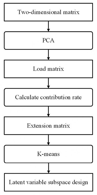
Online monitoring of batch processes combining subspace design of latent variables with support vector data description

Figure 1. Latent variable subspace design flow diagram based on PCA-K-means. PCA: Principal component analysis.

3.2. Online monitoring of batch process based on PCA-MSSVDD

The batch process historical data comprise a three-dimensional data matrix X (I × J × K). Here, I represents the number of batches, J represents the number of variables, and K represents the number of sampling points. First, three-dimensional data matrix X (I × J × K) is expanded into two-dimensional matrix X_B (I × JK) by batch expansion. Then, the data are standardized to mean 0 and variance 1, and the batch expansion X_B (I × JK) is transformed into variable expansion X_V (IK × J). The latent variables are obtained by PCA transformation of X_V (IK × J). On the basis of latent variables, the sliding time window technology and subspace design method are applied to build the SVDD model of the obtained subspace matrix of time slice. The length of all time windows is set to 1 moment. The reason the window length is selected as 1 moment is that, the shorter is the time window, the smaller is the data fluctuation, which can avoid the influence of data fluctuation on the modeling and thus highlight the influence of subspace design on monitoring. When online monitoring, online samples are first mapped to latent variables by PCA model of X_V (IK × J). Then, the monitoring model is selected according to the time. Finally, the fusion method of weighted average is used for monitoring results in different subspaces, where C represents the number of subspaces and DR_c represents the monitoring results of the c-th subspace. The calculation formula is as follows:

(20)

$$ D R=\frac{\sum_{c=1}^{C}\left(D R_{c}\right)^{2}}{\sum_{c=1}^{C} D R_{c}} \\ $$

The flow chart of PCA-MSSVDD is shown in Figure 2. The specific monitoring steps are as follows:

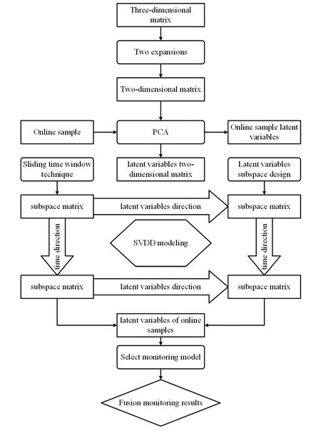
Figure 2. Batch process monitoring flow diagram based on PCA-MSSVDD. PCA-MSSVDD: Principal component analysis - multiple subspace support vector data description; SVDD: support vector data description; PCA: principal component analysis.

The three-dimensional matrix is transformed into the two-dimensional matrix of variable expansion by two expansion techniques.
PCA transform is applied to the two-dimensional matrix of variable expansion.
The sliding time window technique is used to obtain the time slice matrix for the latent variable of the two-dimensional matrix.
The subspace of the latent variable two-dimensional matrix is designed to obtain the results of subspace design.
The SVDD monitoring model for the subspace matrix of latent variable time slice is established.
The latent variables of online samples are obtained by transforming the online samples according to the second PCA model.
The online sample latent variables select the monitoring model according to time.
The subspace monitoring results are fused.

4. EXPERIMENTAL TEST

4.1. Numerical simulation

This paper designs the following numerical simulation models with two subsystems:

(21)

$$ \begin{array}{l} P=\left[\begin{array}{cccccccccccccccc} 1&1&1&1&1&1&1&1&&&&&&&& \\ &1&1&1&1&1&1&1&&&&&&&&\\ &&1&1&1&1&1&1&&&&&&&&\\ &&&1&1&1&1&1&&&&&&&&\\ &&&&1&1&1&1&&&&&&&&\\ &&&&&1&1&1&&&&&&&&\\ &&&&&&1&1&&&&&&&&\\ &&&&&&&1&&&&&&&&\\ &&&&&&&&1&&&&&&&\\ &&&&&&&&1&1&&&&&&\\ &&&&&&&&1&1&1&&&&&\\ &&&&&&&&1&1&1&1&&&&\\ &&&&&&&&1&1&1&1&1&&&\\ &&&&&&&&1&1&1&1&1&1&&\\ &&&&&&&&1&1&1&1&1&1&1&\\ &&&&&&&&1&1&1&1&1&1&1&1\\ \end{array}\right] \\ \end{array}\\ $$

(22)

$$ \begin{array}{l} \boldsymbol{t}_{1}=16 * \text { randi }(10,800,1) \\ \boldsymbol{t}_{2}=15 * \operatorname{randi}(10,800,1) \\ \boldsymbol{t}_{3}=14 * \text { randi }(10,800,1) \\ \boldsymbol{t}_{4}=13 * \text { randi }(10,800,1) \\ \boldsymbol{t}_{5}=12 * \operatorname{randi}(10,800,1) \\ \boldsymbol{t}_{6}=11 * \operatorname{randi}(10,800,1) \\ \boldsymbol{t}_{7}=10 * \operatorname{randi}(10,800,1) \\ \boldsymbol{t}_{8}=9 * \operatorname{randi}(10,800,1) \\ \boldsymbol{t}_{9}=8 * \operatorname{randi}(10,800,1) \\ \boldsymbol{t}_{10}=7 * \text { randi }(10,800,1) \\ \boldsymbol{t}_{11}=6 * \operatorname{randi}(10,800,1) \\ \boldsymbol{t}_{12}=5 * \text { randi }(10,800,1) \\ \boldsymbol{t}_{13}=4 * \text { randi }(10,800,1) \\ \boldsymbol{t}_{14}=3 * \text { randi }(10,800,1) \\ \boldsymbol{t}_{15}=2 * \operatorname{randi}(10,800,1) \\ \boldsymbol{t}_{16}=1 * \operatorname{randi}(10,800,1) \\ \end{array} $$

(23)

$$ \text { noise }=0.5 * \operatorname{randi}(10,800,16) \\ $$

(24)

$$ \boldsymbol{T}=[\begin{array}{llllllllllllllll} \boldsymbol{t}_{1} & \boldsymbol{t}_{2} & \boldsymbol{t}_{3} & \boldsymbol{t}_{4} & \boldsymbol{t}_{5} & \boldsymbol{t}_{6} & \boldsymbol{t}_{7} & \boldsymbol{t}_{8} & \boldsymbol{t}_{9} & \boldsymbol{t}_{10} & \boldsymbol{t}_{11} & \boldsymbol{t}_{12} & \boldsymbol{t}_{13} & \boldsymbol{t}_{14} & \boldsymbol{t}_{15} & \boldsymbol{t}_{16}\end{array}]\\ $$

(25)

$$ x_{i, j}=\sqrt{\boldsymbol{h}_{i} \cdot \boldsymbol{p}_{j}}+\text { noise }_{i, j} \quad i=1,2, \ldots, 800 \quad j=1,2, \ldots, 16 \\ $$

Here, randi (10,800,1) represents a randomly generated column vector with 800 rows and 1 column, and the sample is uniformly distributed between 0 and 10. randi (10,800,16) represents a randomly generated matrix with 800 rows and 16 columns, and the sample of each column obeys a uniform distribution between 0 and 10. x_i,j is the i-th row and the j-th sample, h_i is the i-th row vector in the matrix T, and noise_i,j is the i-th row and the j-th sample.

The gray scale diagram of the extension indicator matrix of the load matrix in the numerical simulation process is shown in Figure 3. The abscissa represents the serial number of the load vector, while the ordinate represents the serial number of the variables in the numerical simulation process. The color of the square in the figure indicates the importance of the process variables to the latent variables: white indicates the most important and black indicates the least important. Therefore, the lighter is the color, the more important are the process variables to the latent variables, and the more obvious are the characteristics. From the gray scale diagram of the extension matrix, it can be clearly seen that Process Variables 1-8 are important to Latent Variables 1, 4, and 12-16. Process Variables 9-16 are important to the remaining latent variables. According to the design knowledge of the numerical model, the latent variables of the numerical simulation model are divided into two subspaces. The design results of the latent variable subspace in the numerical simulation process are shown in Table 1, where Latent Variables 1, 4, and 11-16 form subspace T₁, while Latent Variables 2, 3, and 5-10 form subspace T₂.

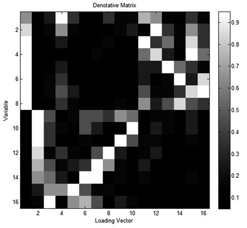
Figure 3. Gray schematic diagram of the denotative matrix in the numerical process.

Table 1

Latent variable subspace design result in the numerical process

Subspace number	Latent variable number
T₁	1, 4, 11, 12, 13, 14, 15, 16
T₂	2, 3, 5, 6, 7, 8, 9, 10

Based on the numerical simulation model, a cross-subsystem local fault is designed, that is, fault signals are introduced into both subsystems to analyze and compare the monitoring performance of SVDD, MSSVDD, and PCA-MSSVDD. The failure results are shown in Table 2. From Time 201 to the end of the process operation, a step fault signal with a size of 16 is introduced into Variable 1; a step fault signal with a magnitude of 3 is introduced into Variable 13; and a step fault signal with a magnitude of 4 is introduced into Variable 15. Such local faults are scattered in different subsystems, which is not conducive to the variable subspace monitoring algorithm detecting variation characteristics.

Table 2

The parameters of the test case in the numerical process

Variable number of the fault signal is introduced	Size of step fault	Time of fault
1	16	201-800
13	3	201-800
15	4	201-800

The comparison of SVDD, MSSVDD, and PCA-MSSVDD in monitoring the numerical process is shown in Table 3. Comparing the false alarm rates shows that the false alarm rate of PCA-MSSVDD is 1.5, slightly higher than the best value of 0. The results show that the missing alarm rate of PCA-MSSVDD is 15.3, which is significantly lower than those of SVDD and MSSVDD (47.0 and 68.5, respectively). The error rate comparison results show that the error rate of PCA-MSSVDD is 11.8, which is obviously better than those of SVDD and MSSD (35.3 and 51.5, respectively). The comparison results of the first time to detect fault shows that the first time to detect fault by PCA-MSSVDD, SVDD, and MSSVDD is the 201st time. Therefore, PCA-MSSVDD has better monitoring effect for local faults scattered in different subsystems.

Table 3

The comparison of SVDD, MSSVDD, and PCA-MSSVDD in monitoring the numerical process

	SVDD	MSSVDD	PCA-MSSVDD
False alarm rate	0	0	1.5
Missed alarm rate	47.0	68.5	15.3
Error rate	35.3	51.5	11.8
First time to detect fault	201	201	201

SVDD: Support vector data description; MSSVDD: multiple subspaces SVDD; PCA-MSSVDD: principal component analysis - multiple subspace support vector data description.

The comparison charts of SVDD, MSSVDD, and PCA-MSSVDD for the test case in monitoring the numerical process is shown in Figure 4. During the whole phase of introducing fault signals, the statistics of PCA-MSSVDD are mostly above the control limit, while only a few of those of SVDD and MSSD are above the control limit.

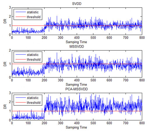
Figure 4. The comparison charts of SVDD, MSSVDD, and PCA-MSSVDD for the test case in monitoring the numerical process. SVDD: Support vector data description; MSSVDD: multiple subspaces SVDD; PCA-MSSVDD: principal component analysis - multiple subspace support vector data description.

The comparison charts of the PCA-MSSVDD subspace for the text case in monitoring the numerical process is shown in Figure 5. It can be clearly seen that most faults are detected in the second subspace, while are few faults are detected in the first subspace.

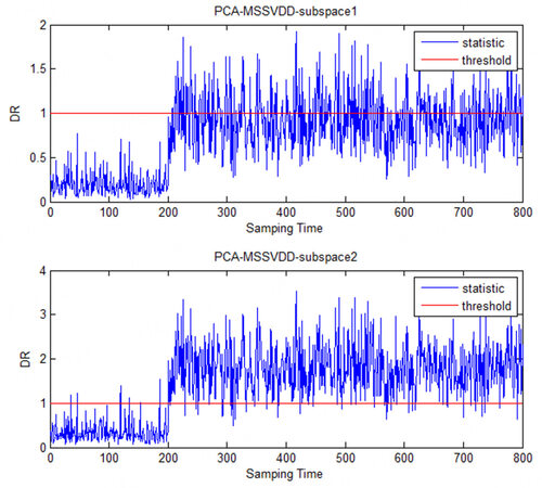
Figure 5. The comparison charts of the PCA-MSSVDD subspace for the text case in monitoring the numerical process. PCA-MSSVDD: Principal component analysis - multiple subspace support vector data description.

4.2. Simulation test of the penicillin fermentation process

The simulation model of the penicillin fermentation process is designed to provide a standard testing platform for data-driven batch process monitoring methods^[22]. Under the normal state set value of process variables, the production cycle of the penicillin fermentation process is set to 400 h, data are recorded once every 0.5 g, and 800 sampling data can be recorded by one simulation^[23]. There is random noise in the simulation model. Under the same initial set value, the data between different batches fluctuate randomly. Therefore, 100 batches of simulation data are collected as a historical reference database.

The gray scale diagram of the extension indicator matrix of the load matrix retained during penicillin fermentation is shown in Figure 6. All features of each latent variable can be clearly seen. The abscissa indicates the serial number of the load vector, while the ordinate indicates the serial number of the process variable. The color of the square in the figure indicates the importance of process variables to latent variables. The lighter is the color, the more important are the process variables to latent variables. In this section, latent variables are also divided into two subspaces according to prior knowledge. Hidden variable subspace design results for the penicillin fermentation process are shown in Table 4, where Hidden Variables 1, 2, and 10-16 form subspace T₁, while Hidden Variables 3-9 form subspace T₂. As shown in Figure 6, the information of Variables 1, 2, and 4 is more projected in the first subspace, while the information of Variables 3, 5, and 7-9 is more projected in the second subspace.

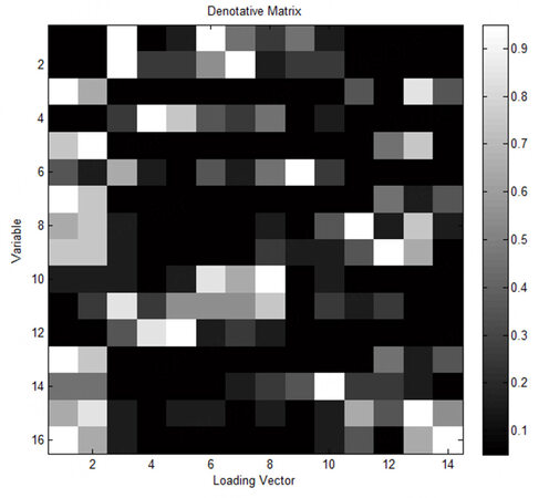
Figure 6. Gray schematic diagram of the denotative matrix in the penicillin fermentation process.

Table 4

Hidden variable subspace design result in the penicillin fermentation process

Subspace number	Latent variable number
T₁	1, 2, 11, 12, 13, 14
T₂	3, 4, 5, 6, 7, 8, 9,10

The simulation of the penicillin fermentation process provides three types of faults: (1) the fault of the ventilation rate variable; (2) the fault of the stirring power variable; and (3) the fault of the glucose flow rate variable. In this paper, six test faults are designed through the simulation test platform to simulate abnormal operation behavior in actual production. The size and types of faults used to test the monitoring algorithm are shown in Table 5.

Table 5

Test cases of the fed-batch penicillin fermentation process

Fault serial number	Failure variable	Variable number	Fault type	Size	Time to detect fault (h)
1	Ventilation rate	1	Step	-1.5(%)	100-400
2	Stirring power	2	Step	-1.5(%)	100-400
3	Glucose flow rate	3	Step	-2.0(%)	100-400
4	Ventilation rate	1	Slope	-0.1	100-400
5	Stirring power	2	Slope	-0.1	100-400
6	Glucose flow rate	3	Slope	-0.001	100-400

The above six kinds of faults are used for monitoring and comparing SVDD, MSSD, and PCA-MASVDD. The comparison of the false alarm rate, missed alarm rate, error rate, and first time to detect fault using SVDD, MSSVDD, and PCA-MSSVDD in monitoring the penicillin fermentation process are shown in Table 6. Comparing the false alarm rates shows that the false alarm rate of PCA-MSSVDD has the optimal value for Faults 4-6. Comparing the missed alarm rate shows that the missed alarm rate of PCA-MSSVDD only has the optimal value in Fault 2. In Faults 1, 2, 4, and 5, the missed alarm rate of PCA-MSSVDD is lower than that of SVDD. In Faults 1, 4, and 5, the missed alarm rate of PCA-MSSVDD is slightly higher than that of MSSVDD. Comparing the error rates shows that the error rate of PCA-MSSVDD has no optimal value. In Faults 1, 2, 4, and 5, the error rate of PCA-MSSVDD is lower than that of SVDD. In Faults 1, 2, 4, and 5, the error rate of PCA-MSSVDD is slightly higher than that of MSSD. In faults 1, 2, 4, and 5, the error rate of PCA-MSSVDD is slightly higher than that of MSSVDD. Comparing the first time to detect fault shows that, Faults 1, 3, 4, and 5, PCA-MSSVDD has the earliest time to detect fault. Therefore, PCA-MSSVDD is more sensitive to fault signals.

Table 6

The comparison of the false alarm rate, missed alarm rate, error rate, and first time to detect fault using SVDD, MSSVDD, and PCA-MSSVDD in monitoring the penicillin fermentation process

	Fault serial number	SVDD	MSSVDD	PCA-MSSVDD
False alarm rate	1	0	0	0.5
	2	0.5	0	2.5
	3	1.5	0.5	2.0
	4	0	0.5	0
	5	0	0	0
	6	0	0	0
Missed alarm rate	1	71.7	25.4	27.6
	2	70.7	39.9	39.9
	3	24.4	33.2	33.2
	4	51.9	38.1	42.2
	5	98.8	94.0	94.5
	6	22.4	23.1	27.9
Error rate	1	53.8	19.1	20.8
	2	53.2	30.0	30.6
	3	18.7	25.1	25.5
	4	39.0	28.7	31.7
	5	74.2	70.6	71.0
	6	16.8	17.3	21.0
First time to detect fault	1	122	100	100
	2	111	101	105
	3	142	137	121
	4	141	138	125
	5	397	171	106
	6	164	159	161

SVDD: Support vector data description; MSSVDD: multiple subspaces SVDD; PCA-MSSVDD: principal component analysis - multiple subspace support vector data description.

The comparison charts of SVDD, MSSVDD, and PCA-MSSVDD for Fault 3 in monitoring the penicillin fermentation process are shown in Figure 7. At about the 120th hour, PCA-MSSVDD has a peak value and a fault can be detected. At this time, the statistics of SVDD and MSSVDD have not exceeded the control limit. The statistics of SVDD and MSSVDD fall back to the position below the control limit after the 350th hour, while the statistics of PCA-MSSVDD are not below the control limit, and faults can still be detected.

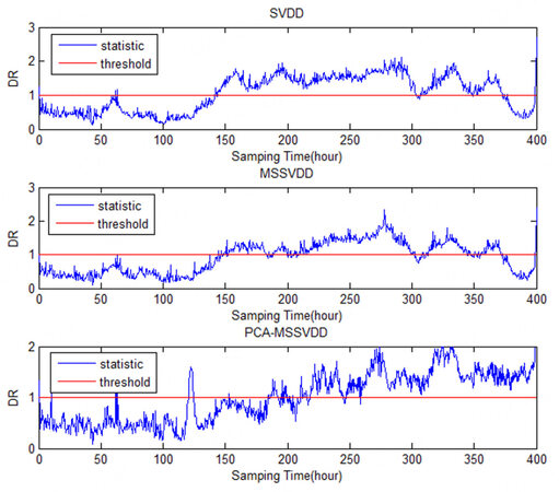
Figure 7. The comparison charts of SVDD, MSSVDD, and PCA-MSSVDD for Fault 3 in monitoring the penicillin fermentation process. SVDD: Support vector data description; MSSVDD: multiple subspaces SVDD; PCA-MSSVDD: principal component analysis - multiple subspace support vector data description.

The comparison charts of SVDD, MSSVDD, and PCA-MSSVDD for Case 6 in monitoring the penicillin fermentation process are shown in Figure 8. From the 150th hour to the 200th hour, the statistics of SVDD, MSSD, and PCA-MSSD all have an upward trend. However, the statistics of PCA-MSSD have a small jump signal, which exceeds the control limit and can detect the fault earlier.

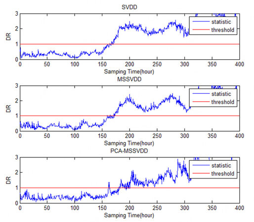
Figure 8. The comparison charts of SVDD, MSSVDD, and PCA-MSSVDD for Case 6 in monitoring the penicillin fermentation process. SVDD: Support vector data description; MSSVDD, multiple subspaces SVDD; PCA-MSSVDD: principal component analysis - multiple subspace support vector data description.

Combining the above two monitoring comparison charts, Figure 7 shows that PCA-MSSVDD has a better monitoring effect than MSSVDD at about the 125th hour and from the 350th hour to the end of the process; however, MSSVDD has a better monitoring effect than PCA-MSSVDD from the 150th hour to the 200th hour. Figure 8 shows that PCA-MSSVDD can detect faults earlier, but MSSVDD has a better monitoring effect than PCA-MSSVDD around the 200th hour. Therefore, the simulation test of the penicillin fermentation process shows that PCA-MSSVDD has better fault detection capability than MSSD in some cases but a worse one in other cases.

The comparison charts of PCA-MSSVDD subspace for Faults 1-6 in monitoring the penicillin fermentation process are shown in Figures 9-14. It can be easily seen that Faults 1 and 4 both occur on Variable 1, so they can be detected in the second subspace. Fault 2 occurs on Variable 2, so it can be detected in the second subspace. Faults 3 and 6 are both faults occurring on Variable 3, so they can be detected in the first subspace. The information of Variables 1 and 2 is mainly projected into the second subspace, while the information of Variable 3 is mainly projected into the first subspace.

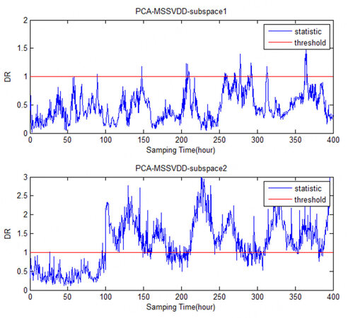
Figure 9. The comparison charts of the PCA-MSSVDD subspace for Fault 1 in monitoring the penicillin fermentation process. PCA-MSSVDD: Principal component analysis - multiple subspace support vector data description.

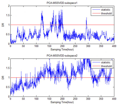
Figure 10. The comparison charts of the PCA-MSSVDD subspace for Fault 2 in monitoring the penicillin fermentation process. PCA-MSSVDD: Principal component analysis - multiple subspace support vector data description.

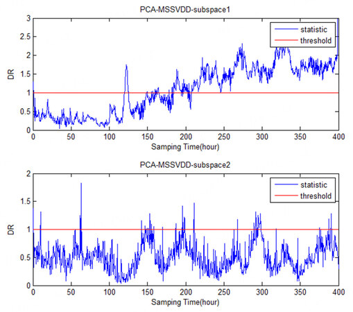
Figure 11. The comparison charts of the PCA-MSSVDD subspace for Fault 3 in monitoring the penicillin fermentation process. PCA-MSSVDD: Principal component analysis - multiple subspace support vector data description.

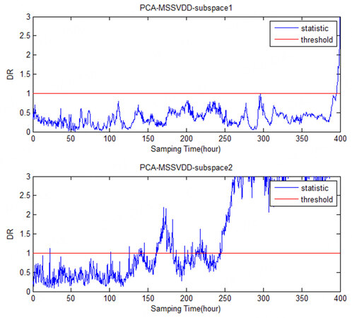
Figure 12. The comparison charts of the PCA-MSSVDD subspace for Fault 4 in monitoring the penicillin fermentation process. PCA-MSSVDD: Principal component analysis - multiple subspace support vector data description.

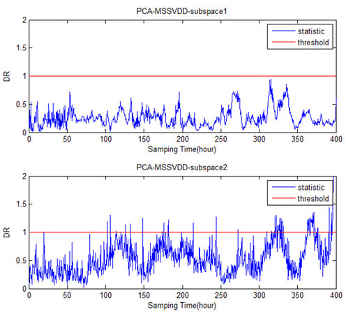
Figure 13. The comparison charts of the PCA-MSSVDD subspace for Fault 5 in monitoring the penicillin fermentation process. PCA-MSSVDD: Principal component analysis - multiple subspace support vector data description.

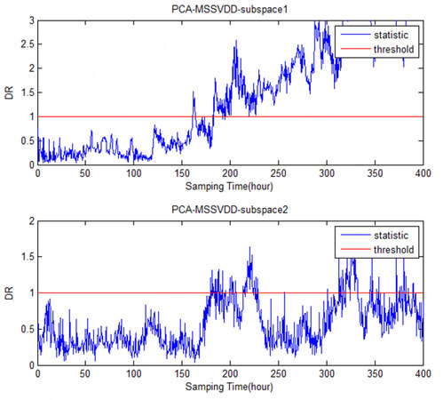
Figure 14. The comparison charts of the PCA-MSSVDD subspace for Fault 6 in monitoring the penicillin fermentation process. PCA-MSSVDD: Principal component analysis - multiple subspace support vector data description.

Using the above six test faults of the penicillin fermentation process simulation, the comparison of the false alarm rate of the penicillin fermentation process monitoring based on multi-way principal component analysis (MPCA)^[24], multi-way independent component analysis (MICA)^[25], batch dynamic principal component analysis (BDPCA)^[26], mixture probabilistic principal component analysis (MPPCA)^[27], and PCA-MSSVDD is shown in Table 7. For Faults 4-6, PCA-MSSVDD has the most merit. Based on MPCA, MICA, BDPCA, MPPCA, and PCA-MSSVDD, the false negative rate of the penicillin fermentation process monitoring is shown in Table 8. For Faults 1-3, PCA-MSSVD has the optimal value. Based on MPCA, MICA, BDPCA, MPPCA, and PCA-MSSVDD, the monitoring error rate of the penicillin fermentation process is shown in Table 9. For Faults 1-3, PCA-MSSVDD has the optimal value. The first time to detect fault of the penicillin fermentation process monitoring based on MPCA, MICA, BDPCA, MPPCA, and PCA-MSSVDD is shown in Table 10. For Fault 1, PCA-MSSVDD has the optimal value. Therefore, in some test failures, PCA-MSSVDD has better monitoring results.

Table 7

The comparison of the false alarm rate using MPCA, MICA, BDPCA, MPPCA, and PCA-MSSVDD in monitoring the penicillin fermentation process

Fault serial number	MPCA		MICA		BDPCA		MPPCA		PCA-MSSVDD
Fault serial number	T²	SPE	I²	SPE	T²	SPE	T²	SPE	DR
1	0	0.5	3.5	1.0	1.0	6.5	0	0	0.5
2	0	12.0	1.5	0	2.5	18.5	2.5	0	2.5
3	0	5.0	3.5	17.0	0.5	11.5	0.5	0.5	2.0
4	0	0	1.5	0.5	0	6.5	0	0	0
5	0	0	1.5	0	0	7.0	0	0	0
6	0	0	2.0	0	0	5.5	0	0	0

MPCA: Multi-way principal component analysis; MICA: multi-way independent component analysis; BDPCA: batch dynamic principal component analysis; MPPCA: mixture probabilistic principal component analysis; PCA-MSSVDD: principal component analysis - multiple subspace support vector data description.

Table 8

The comparison of the missed alarm rate using MPCA, MICA, BDPCA, MPPCA, and PCA-MSSVDD in the monitoring the penicillin fermentation process

Fault serial number	MPCA		MICA		BDPCA		MPPCA		PCA-MSSVDD
Fault serial number	T²	SPE	I²	SPE	T²	SPE	T²	SPE	DR
1	100	54.2	99.0	40.5	33.6	71.5	48.9	95.1	27.6
2	100	68.2	98.6	88.8	44.8	72.1	75.2	95.8	39.9
3	88.3	51.5	92.8	97.5	49.0	77.6	42.5	42.5	33.2
4	100	48.4	98.1	39.9	47.1	66.3	47.5	96.5	42.2
5	100	96.6	99.1	86.8	98.3	91.0	98.6	99.3	94.5
6	77.8	25.4	86.0	90.3	31.8	76.8	23.2	22.1	27.9

Table 9

The comparison of the error rate using MPCA, MICA, BDPCA, MPPCA, and PCA-MSSVDD in monitoring the penicillin fermentation process

Fault serial number	MPCA		MICA		BDPCA		MPPCA		PCA-MSSVDD
Fault serial number	T²	SPE	I²	SPE	T²	SPE	T²	SPE	DR
1	75.1	40.8	75.2	30.7	25.5	55.4	36.7	71.5	20.8
2	75.1	54.2	74.5	66.7	34.3	58.9	57.1	72.0	30.6
3	66.3	40.0	70.6	77.5	36.9	61.2	32.1	32.1	25.5
4	75.1	36.3	74.1	30.1	35.4	51.5	35.7	72.5	31.7
5	75.1	72.6	74.8	65.2	73.9	70.2	74.1	74.6	71.0
6	58.5	19.1	65.1	67.8	23.9	59.1	17.5	16.6	21

Table 10

The comparison of the first time to detect fault using MPCA, MICA, BDPCA, MPPCA, and PCA-MSSVDD in monitoring the penicillin fermentation process

Fault serial number	MPCA		MICA		BDPCA		MPPCA		PCA-MSSVDD
Fault serial number	T²	SPE	I²	SPE	T²	SPE	T²	SPE	DR
1	/	100	397	100	100	100	100	127	100
2	111	101	105	101	104	101	100	111	105
3	142	137	121	137	106	106	104	142	121
4	/	142	395	163	166	112	142	352	125
5	397	171	106	102	102	108	102	397	106
6	334	164	328	194	171	148	167	166	161

5. CONCLUSIONS

In this paper, a batch process monitoring algorithm based on PCA-MSSVDD is proposed by combining latent variable subspace design with SVDD. Subspace monitoring by PCA and K-means can effectively reduce the risk of inundation of variation features; using SVDD to establish subspace monitoring model can make the proposed method applicable to any non-Gaussian process.

Through the numerical simulation process and penicillin fermentation simulation process test, the comparison results between PCA-MSSVDD and SVDD show that the subspace monitoring algorithm can effectively reduce the risk of variation characteristics being submerged and improve the monitoring performance. The comparison results between PCA-MSSVDD and MSSVDD show that the fault detection capability of PCA-MSSVDD may be higher than that of MSSVDD or lower than that of MSSVDD. For local failures of weakly correlated variables, the proposed PCA-MSSVDD method will have better results, while, for strongly correlated variables, the MSSVDD method will have better results, and both methods have better performance than SVDD.

DECLARATIONS

Authors contributions

The author contributed solely to the article.

Availability of data and material

Not applicable.

Financial support and sponsorship

Opening Project of Shanghai Trusted Industrial Control Platform (TICPSH202103003-ZC).

Conflicts of interest

The author declared that there are no conflicts of interest.

Ethical approval and consent to participate

Not applicable.

Consent for publication

Not applicable.

Copyright

REFERENCES

1. Zhao C, Huang B. A full-condition monitoring method for nonstationary dynamic chemical processes with cointegration and slow feature analysis. AIChE J 2018;64:1662-81.

2. Qin Y, Zhao C, Gao F. An iterative two-step sequential phase partition (ITSPP) method for batch process modeling and online monitoring. AIChE J 2016;62:2358-73.

3. Zhang S, Zhao C. Slow-feature-analysis-based batch process monitoring with comprehensive interpretation of operation condition deviation and dynamic anomaly. IEEE Trans Ind Electron 2019;66:3773-83.

4. Yin S, Li X, Gao H, Kaynak O. Data-based techniques focused on modern industry: An overview. IEEE Trans Ind Electron 2015;62:657-67.

5. Ge Z, Song Z, Deng SX, Huang B. Data mining and analytics in the process industry: the role of machine learning. IEEE Access 2017;5:20590-616.

6. Yuan X, Wang Y, Yang C, et al. Weighted linear dynamic system for feature representation and soft sensor application in nonlinear dynamic industrial processes. IEEE Trans Ind Electron 2018;65:1508-17.

7. Song B, Shi H. Fault detection and classification using quality-supervised double-layer method. IEEE Trans Ind Electron 2018;65:8163-72.

8. Peng X, Tang Y, Du W, Qian F. Multimode process monitoring and fault detection: a sparse modeling and dictionary learning method. IEEE Trans Ind Electron 2017;64:4866-75.

9. He Y, Le Z, Ge Z, et al. Distributed model projection based transition processes recognition and quality-related fault detection. Chemometr Intell Lab 2016;159:69-79.

10. Lv Z, Yan X, Jiang Q. Batch process monitoring based on just-in-time learning and multiple-subspace principal component analysis. Chemometr Intell Lab 2014;137:128-39.

11. Jiang Q, Ding SX, Wang Y, Yan X. Data-driven distributed local fault detection for large-scale processes based on the GA-regularized canonical correlation analysis. IEEE Trans Ind Electron 2017;64:8148-57.

12. Lv Z, Yan X. Hierarchical support vector data description for batch process monitoring. Ind Eng Chem Res 2016;55:9205-14.

13. Jian H, Yan X. Gaussian and non-Gaussian double subspace statistical process monitoring based on principal component analysis and independent component analysis. Ind Eng Chem Res 2015;54:1015-27.

14. Tong C, Lan T, Shi X. Double-layer ensemble monitoring of non-gaussian processes using modified independent component analysis. ISA Trans 2017;68:181-8.

15. Lv Z, Jiang Q, Yan X. Batch process monitoring based on multisubspace multiway principal component analysis and time-series bayesian inference. Ind Eng Chem Res 2014;53:6457-66.

16. Ge Z, Xie L, Kruger U, et al. Sensor fault identification and isolation for multivariate non-Gaussian processes. J Process Contr 2009;19:1707-15.

17. Ge Z, Gao F, Song Z. Batch process monitoring based on support vector data description method. J Process Contr 2011;21:949-59.

18. Lv Z, Yan X, Jiang Q, et al. Just-in-time learning-multiple subspace support vector data description used for non-Gaussian dynamic batch process monitoring. J Chemometr 2019:e3134.

19. Jiang Q, Yan X. Just-in-time reorganized PCA integrated with SVDD for chemical process monitoring. AIChE J 2014;60:949-65.

20. Hartigan J A, Wong M A. A K-means clustering algorithm. Appl Stat 1979;28:100-8.

21. Jiang Q, Yan X. Parallel PCA-KPCA for nonlinear process monitoring. Control Eng Pract 2018;80:17-25.

22. Birol G, Ündey C, Çinar A. A modular simulation package for fed-batch fermentation: penicillin production. Comput Chem Eng 2002;26:1553-65.

23. Lv Z, Yan X, Jiang Q. Batch process monitoring based on self-adaptive subspace support vector data description. Chemometr Intell Lab 2017;170:25-31.

24. Nomikos P, Macgregor JF. Multi-way partial least squares in monitoring batch processes. Chemometr Intell Lab Syst 1995;30:97-108.

25. Lee JM, Yoo C, Lee IB. On-line batch process monitoring using different unfolding method and independent component analysis. J Chem Eng Japan 2003;36:1384-96.

26. Chen J, Liu K. On-line batch process monitoring using dynamic PCA and dynamic PLS models. Chem Eng Sci 2002;57:63-75.

27. Raveendran R, Huang B. Mixture probabilistic PCA for process monitoring-collapsed variational bayesian approach. IFAC-PapersOnLine 2016;49:1032-7.

Cite This Article

Export citation file: BibTeX | RIS

OAE Style

Lv Z. Online monitoring of batch processes combining subspace design of latent variables with support vector data description. Complex Eng Syst 2021;1:4. http://dx.doi.org/10.20517/ces.2021.02

AMA Style

Lv Z. Online monitoring of batch processes combining subspace design of latent variables with support vector data description. Complex Engineering Systems. 2021; 1(1): 4. http://dx.doi.org/10.20517/ces.2021.02

Chicago/Turabian Style

Lv, Zhaomin. 2021. "Online monitoring of batch processes combining subspace design of latent variables with support vector data description" Complex Engineering Systems. 1, no.1: 4. http://dx.doi.org/10.20517/ces.2021.02

ACS Style

Lv, Z. Online monitoring of batch processes combining subspace design of latent variables with support vector data description. Complex. Eng. Syst. 2021, 1, 4. http://dx.doi.org/10.20517/ces.2021.02

About This Article

Copyright

© The Author(s) 2021. Open Access This article is licensed under a Creative Commons Attribution 4.0 International License (https://creativecommons.org/licenses/by/4.0/), which permits unrestricted use, sharing, adaptation, distribution and reproduction in any medium or format, for any purpose, even commercially, as long as you give appropriate credit to the original author(s) and the source, provide a link to the Creative Commons license, and indicate if changes were made.

Data & Comments

Data

Views

1465

Downloads

681

Citations

Comments

Comments

Comments must be written in English. Spam, offensive content, impersonation, and private information will not be permitted. If any comment is reported and identified as inappropriate content by OAE staff, the comment will be removed without notice. If you have any queries or need any help, please contact us at support@oaepublish.com.