
Prediction of sea temperature using temporal convolutional network and LSTM-GRU network

 , ...
, ... Abstract
The ocean is a complex system. Ocean temperature is an important physical property of seawater, so studying its variation is of great significance. Two kinds of network structures for predicting thermocline time series data are proposed in this paper. One is the LSTM-GRU hybrid neural network model, and the other is the temporal convolutional network (TCN) model. The two networks have obvious advantages over other models in accuracy, stability, and adaptability. Compared with the traditional auto-regressive integrate moving average model, the proposed method considers the influence of temperature history, salinity, depth, and other information. The experimental results show that TCN performs better in prediction accuracy, while LSTM-GRU can better predict abnormal data and has higher robustness.
Keywords
1. INTRODUCTION
As global warming continues to intensify, the living environment of humankind is facing increasingly severe challenges, and ocean-related research has also received growing attention. The ocean plays an important role in regulating global temperature. However, the ocean is an open and complex system. Ocean research always includes seawater, dissolved and suspended substances, organisms, submarine sediments, the lithosphere, the atmospheric boundary layer, and estuarine and coastal zones. Seawater temperature is an important parameter in ocean research. Affected by the latitude and geographic environment, the ocean temperature is highly unstable in time and space. Ocean temperature affects rainfall and seawater evaporation around the world and affects sea-air heat exchange[1]. Thus, the study of ocean temperature prediction methods can provide more reference data for predicting climate and meteorological changes, thereby promoting atmospheric and ocean sciences, expanding the scope and time of natural disaster forecasting, and reducing the losses caused by natural disasters to humans as much as possible. The change in ocean temperature will affect the abundance of marine species and the production of marine organisms. Therefore, predicting ocean temperature is also conducive to fishery production scheduling and promotes the fishery economy.
Argo is an international program that uses profiling floats to observe temperature, salinity, currents, and, recently, bio-optical properties in the oceans; it has been operational since the early 2000s[2]. The collected data are used in climate and oceanographic research. Argo originally planned to put 3000 buoys in international waters and establish a global ocean observation network with a density of buoys with an average distance between buoys of 3 km × 3 km. There are three main tasks: Argo core, measuring temperature, salinity, and pressure above 2000 m; deep Argo, measuring temperature, salinity, and pressure above 6000 m; and BGC-Argo, measuring temperature, salinity, pressure, pH, nitrate, chlorophyll, backscatter, oxygen content, and irradiance at a water depth of above 2000 m.
The Argo dataset provides the basis for marine research. Researchers use traditional physical models and machine learning methods to predict ocean temperature. In previous work, we proposed an SVR-based method to predict ocean temperature[3]. We redefined the thermocline by using the information entropy method[4,5] and analyze the association of the temperature and salinity data of seawater[6]. Some scholars also put forward the long short-term memory (LSTM) network and the gated recurrent unit (GRU), their improved algorithm, making a breakthrough in temperature prediction. Based on those studies, we continue to discuss the temperature prediction in this paper. We propose two temperature time-series prediction methods, and our contributions are as follows:
(1) We propose an LSTM-GRU hybrid neural network model and a model based on Temporal Convolutional Networks (TCNs). We compare them with traditional LSTM, GRU, and TCN, and the two networks surpassed them in experiments. The explanatory variable score of both exceeded 0.98.
(2) We evaluated the LSTM-GRU model and TCN-based model to predict data with abnormal data inputs. In the normal data, the TCN-based model works best. However, it is easy to predict abnormal temperatures while inputting insufficient data. The explanatory variable score result of LSTM-GRU can reach 0.85, which has high robustness.
This paper is arranged as follows. Section 2 introduces the application of Argo buoys and the current research status of ocean temperature prediction. Section 3 gives a detailed introduction to the LSTM model, GRU model, TCN, and the model proposed in this paper. Then, in Section 4, a comparison is made among several models, and we also evaluate the LSTM-GRU and TCN-based methods with abnormal data. Section 5 summarizes the work in this paper and looks forward to the future.
2. PRELIMINARY
2.1 Sea surface temperature predict
Sea surface temperature (SST) is an important factor affecting water vapor exchange and heat flow. Therefore, ocean temperature prediction has been considered by many scholars. SST can be divided into two categories in the prediction of ocean temperature: one is the numerical model based on physics, and the other is the data-driven model based on data analysis. In the traditional method, Xue et al.[7] proposed a Markov model to predict the temperature along the tropical Pacific. Based on linear Prediction,
For deep learning methods, Tangang et al.[11] first proposed a neural network model to predict the seasonal ocean temperature anomaly in the tropical Pacific in 1997. Mahonggo and Deo[12] used the method based on the differential autoregressive moving average model and different neural network models to predict sea surface temperature change along the East African coast. Bhaskaran et al.[13] proposed the neural network model to experiment on various ocean datasets and used the nonlinear activation function of multi-layer perceptron to solve the nonlinear problem in the data. Zhang and Wang[1] proposed an LSTM neural network with a fully connected layer to complete ocean temperature prediction. LSTM layer was used to model the time series relationship of ocean data, and the results of the LSTM layer were mapped to the final prediction through the fully connected layer[14]. Yang et al.[15] proposed a CFCC-LSTM (combined fully connected network and convolution neural network) model, making ocean temperature prediction into series prediction problems. They predicted the ocean surface temperature of the Bohai Sea through a complete LSTM layer and a convolution layer[15]. The existing methods show that the method based on time series data effectively predicts ocean temperature, and the LSTM and its improved algorithm show good effect and adaptability in the simulation experiment.
2.2 Auto-regressive integrate moving average model
The marine time series models include the Gaussian, auto-regressive moving average, auto-regressive integrate moving average, Markov chain, and hidden Markov models[16].
The auto-regressive integrate moving average (ARIMA) model is one of the most common statistical models for time series prediction. ARIMA(p, d, q) is composed of three parts: AR is the auto-regressive model, which means that the value of a specific time point at present is equal to the value of several specific time points in the past. Integrate (I) calculates the difference between t time and t-1 time in the time series called first-order difference series. By calculating the first-order difference sequence, the different sequences of other orders can be obtained[17]. Moving average is a regression model derived to compute the regression between the value of certain characteristic points and the prediction errors of several past characteristic time points. The above three parts constitute the ARIMA(p, d, q) model, where p and q represent the order of the auto-regressive model and moving average model, respectively. d is the degree of differencing which is the number of times the data have subtracted past values. γiand θi represent the correlation coefficients of the auto-regressive model and moving average model. μ is a constant and εi represents the white noise.
2.3 LSTM, GRU and TCN
LSTM is an artificial recurrent neural network (RNN) architecture[18] used in the field of deep learning. Unlike standard feedforward neural networks, LSTM has feedback connections which can process not only single data points but also entire sequences of data. GRUs, introduced in 2014 by Cho et al.[19], are a gating mechanism similar to LSTM[20]. In 2015, Lea et al.[21] first proposed TCNs for video-based action segmentation. The conventional process includes two steps: first, extract low-level features using CNN that encode spatial-temporal information. Second, input these feature maps into an RNN classifier that captures high-level temporal information. The main disadvantage is that it requires two separate models. TCN provides a unified approach to capture both levels of information hierarchically.
3. MARINE TEMPERATURE PREDICTION MODEL BASED ON LSTM-GRU AND TCN MODEL
3.1 LSTM and GRU
When predicting time-series data, traditional fully connected neural networks are weak. RNNs can process time-series data. The essential characteristics of RNNs are both an internal feedback connection and a feedforward connection between the processing units[19]. The LSTM network is a special RNN model whose structural design solves long-term dependence issues. The key of LSTM is the cell state to save current status and pass it to the next moment. The LSTM model is shown in Figure 1.
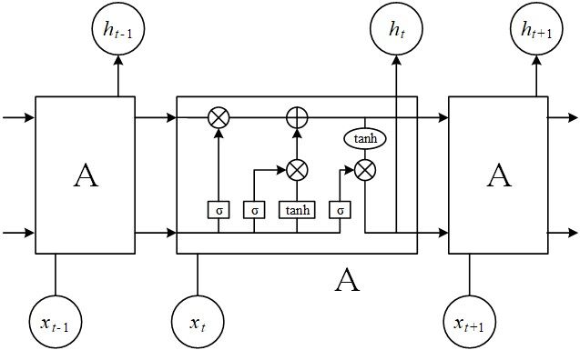
Figure 1. The LSTM model diagram. LSTM: Long short-term memory.
The forget gate in LSTM is used to determine which parts of the input information will be forgotten, as shown in Figure 1. The forget gate includes a sigmoid neural network layer and a bitwise multiplication operation. The forget gate outputs a value between 0 and 1. The higher is the value, the greater is the information obtained by the upper layer[22]. The function of the LSTM memory gate is exactly the opposite of the forget gate, and it decides which information of the input is retained. The LSTM memory gate includes the sigmoid neural network and the tanh neural network layers. The function of the LSTM output gate is to determine the content of the output. The output gate only contains the tanh function, and the output result will also be sent to the next node as the input[23]. GRU is a variant of LSTM. GRU gets rid of the state unit and uses the hidden state to convey information[24]. GRU has only two doors: reset gate and update gate. The reset gate obtains the gate control state through the state ht-1 transmitted by the previous node and the input of the current node. Furthermore, the two steps of forgetting and remembering will be carried out simultaneously in the update gate. That is, only one gate can be used for both forgetting and remembering.
3.2 Temporal convolutional network
The TCN was first proposed by Lea et al.[21] in 2016. At that time, they were researching video action segmentation. Generally speaking, this conventional process includes two steps: first, use CNN to encode spatiotemporal information to calculate low-level features. Second, input these low-level features into a decoder to capture high-level temporal information. Figure 2 shows the structure of TCN.
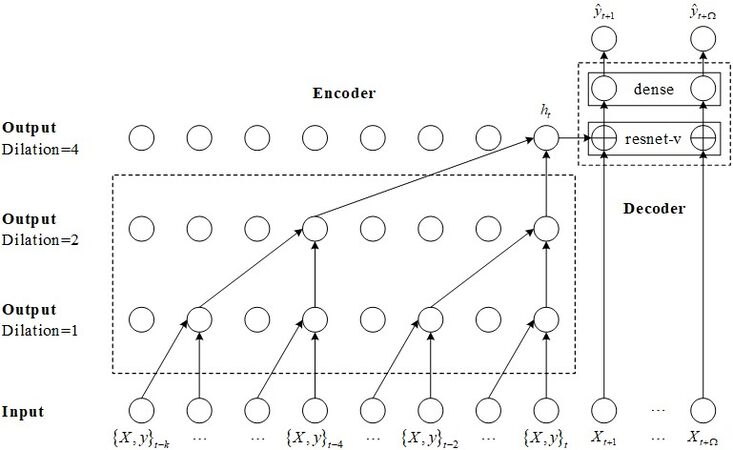
Figure 2. Structure of TCN. TCN: Temporal convolutional network.
Several structures of the TCN model, e.g., causal convolution, dilated convolutions, and the residual block, are image-oriented convolutional neural networks. Causal convolution builds neural networks based on statistical equations [Equation (2)]. For the sequence modeling problem, yt is predicted according to x1... xt and y1... yt-1 to make yt close to the actual value:
Based on causal convolution, dilated convolutions skip part of the input (the isolated circles in Figure 2) to apply the filter to the larger region. It is equivalent to generating a larger filter from the original filter by adding zero. The residual network has a very strong expression ability in computer vision. Introducing residual modules into a temporal convolution network can solve the problem of gradient disappearance. The shallow network can be easily extended to the deep network by the residual module. Different from the RNN structure, TCN can be processed at large scale in parallel. Therefore, the network speed is faster in training and verification. At the same time, the gradient dispersion and gradient explosion problems in RNN are avoided.
3.3 Model structure
Firstly, we propose a hybrid model based on LSTM and GRU, establishing a TCN network model.
The LSTM unit controls the amount of new memory content added to the memory cell independently from the forget gate. The GRU controls the information flow from the previous activation when computing the new, candidate activation, but it does not independently control the amount of added candidate activation (the control is tied via the update gate). LSTM has a talent in new data, but deep LSTM networks always lead to overfitting. GRU concentrates on short old data, and it is at lower risk of overfitting. Thus, we combine these advantages and propose a hybrid network.
The LSTM-GRU hybrid neural network constructed in this paper has five layers. The first layer is the LSTM neural network layer, which contains 30 hidden neurons; the second to fourth layers are the GRU neural network layers, and the numbers of neurons are 24, 6, and 3, respectively; and the fifth layer is a fully connected layer.
Referring to the model structure of the residual network, we design the TCN network structure shown in Figure 3.
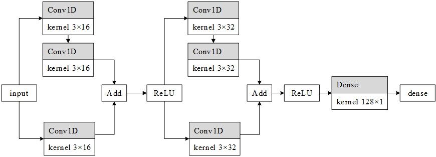
Figure 3. Structure of the proposed model.
The network includes two improved ResNet units. Each unit of the network contains two branches. The first branch contains two convolution layers, and the second branch contains one convolution layer. Each convolution layer of the first unit contains 16 kernels, and the second convolution layer contains 32 kernels. In the second layer of convolution kernels, we set the dilated parameter to 2.
Moreover, we also add two networks for comparison. The first contains 1 unit with 16 convolution kernels. The second contains three units (16, 32, and 64 convolution core), and the dilated number is 1, 2, and 4, respectively. We also compare the network with the traditional TCN, and the experimental results are shown in Section 4.
4. EXPERIMENTS
4.1 Experimental data
The data used in this article were derived from the “Argo (V3.0)” and include over 2.15 million temperature, salinity, and depth profile data obtained from more than 15,000 automatic observation profile buoys worldwide from July 1997 to March 2021. The files in the original dataset are stored according to the buoy number and contain longitude, latitude, pressure, temperature, and salinity. This paper selects eight months of ocean data from April to December 2020 for ocean temperature prediction. After preprocessing, there are 94,075 data items. The data in the original dataset are stored according to the buoy number, each number corresponds to a unique buoy, and the position of each buoy is uniquely determined. This paper only predicts the temperature of the ocean surface. Thus, we only selected the ocean data within 10 m from the sea level, organized the extracted effective data, and stored them again according to the buoy number. This paper divides 90% of the dataset into the training set and 10% in the validation set. The experiments used the following environment: Intel Core i7 7700, 16 GB RAM, RTX 2080TI, Ubuntu 16.04, Python 3.7.4, and TensorFlow 1.13.1. The linear normalization method was adopted to normalize the original data. The batch size was chosen as 100.
4.2 Model evaluation index
In this paper, explained variance score (EVS) and root mean square error (MSE), commonly used in regression models, are selected as the evaluation indicators of the model. The formula for EVS is as follows:
Var is Variance, the square of the standard deviation. ŷ represents the prediction, and y represents the true value. The value range of EVS is [0, 1]. The closer it is to 1, the more the independent variable can explain the variance change of the dependent variable. The smaller the value is, the worse the effect is. MSE is the ratio of the square sum of the deviation between the observed and actual values to the number of samples. The formula is as follows:
MSE is a loss function in linear regression. Under the same conditions, the smaller is the value, the higher is the accuracy of the prediction model.
4.3 Experimental results
4.3.1 ARIMA model prediction performance analysis
The ARIMA model can only predict ocean temperature for a single buoy. From the time perspective, it can only predict ocean temperature and cannot predict ocean temperature in different spaces. When the model parameters are the same, the prediction accuracy of the ARIMA model for different buoys is quite different. The prediction of the ARIMA model is shown in Figure 4. The red line in the figure represents the true value of the ocean temperature recorded by the buoy, while the blue line represents the predicted temperature. The abscissa is the serial number of the selected 80 test points, the ordinate is the temperature, and the unit is degrees Celsius.
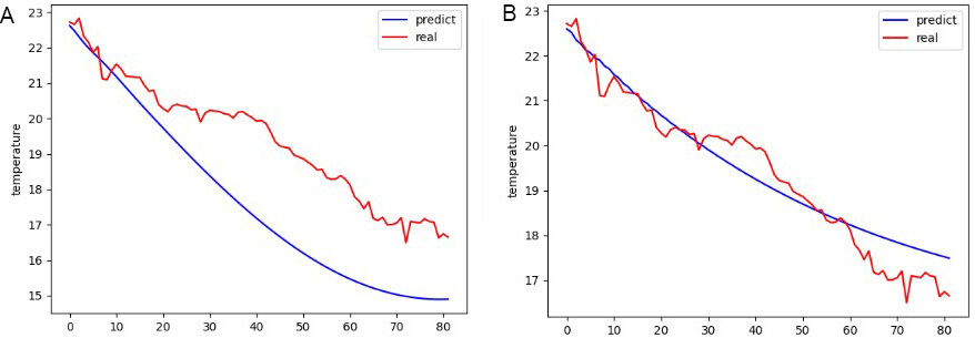
Figure 4. ARIMA model prediction effect diagram. ARIMA: Auto-regressive integrate moving average.
The prediction effect of the ARIMA model in Figure 4 corresponds to MSE of 0.23, and the model running time is about 6 s; the prediction effect of the ARIMA model in Figure 2 corresponds to MSE of 3.81, and the model running time is about 1-2 s. We can draw the following conclusions: (1) When the model parameters are the same, the accuracy of the ARIMA model for the ocean temperature prediction of different buoys varies greatly; and (2) the ARIMA model cannot accurately predict the ocean temperature but can only predict its general trend.
4.3.2 Comparative analysis of prediction performance of neural network models
The neural network model can predict the ocean temperature of all buoys at the same time. We compared LSTM[14], GRU[25], LSTM-GRU, and TCN. The compared TCN network is presented in[26]. The parameters of networks are shown in Table 1.
Networks’ structure and parameters
| Layers/units | Parameters | ||||
| 1 | 2 | 3 | 4 | ||
| LSTM GRU LSTM-GRU TCN-R1 TCN-R2 TCN-R3 TCN-C1 TCN-C2 TCN-C3 TCN-D1 TCN-D2 | 25 25 30 16 × 3 (1) 16 × 3 (1) 16 × 3 (1) 16 × 3 (1) 16 × 3 (1) 16 × 3 (1) 16 × 3 (2) 16 × 3 (1) | 25 25 24 - 32 × 3 (2) 32 × 3 (2) - 32 × 3 (1) 32 × 3 (1) - 32 × 3 (2) | - - 6 - - 64 × 3 (4) - - 64 × 3 (1) - - | - - 3 - - - - - - - - | 8626 6476 9412 1745 8049 32,945 417 1617 3793 401 1585 |
LSTM, GRU, and LSTM-GRU represent the three RNN networks mentioned in Section 3. TCN-R is the TCN network with improved ResNet modules. Moreover, we also label the three traditional TCN casual networks as TCN-C and two TCN casual networks with dilated convolution as TCN-C. The number on the left is the number of convolution kernels, and the right is the kernel size. The number of brackets is the dilated number. The EVS and RMSE of each prediction result are shown in Table 2 and Figure 5. To verify the stability of the prediction results of the neural network model, ten prediction experiments were performed for each neural network model.
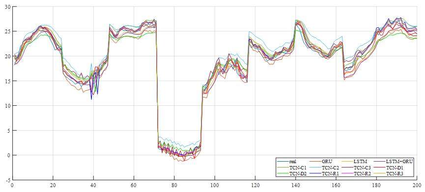
Figure 5. Predictions of all models. LSTM: Long short-term memory; GRU: gated recurrent unit; TCN: temporal convolutional network.
The EVS and MSE of prediction results on the models
| Model | EVS | MSE |
| LSTM GRU LSTM-GRU TCN-R1 TCN-R2 TCN-R3 TCN-C1 TCN-C2 TCN-C3 TCN-D1 TCN-D2 | 0.9564 0.9743 0.9811 0.8978 0.9879 0.9878 0.9797 0.9642 0.9661 0.9573 0.9631 | 3.5275 2.4345 1.6790 8.2182 0.9987 1.0028 1.9759 3.6824 2.7592 4.7414 3.1562 |
In Table 2, we can see that the EVS of the LSTM-GRU hybrid network is lower than those of LSTM and GRU, indicating that the performance of the hybrid network is better than that of a single network. The TCN network with RESNET has the lowest error, which is better than the traditional method and the traditional TCN method. The error of R3 is close to that of R2, which indicates that increasing RESNET units cannot increase the network accuracy. R2 has fewer parameters, which is more suitable for Argo temperature prediction. Although R3 has more network parameters than R2, overfitting and gradient disappearance occur. Therefore, the more parameters are uncertain, the better the effect will be.
In Figure 5, the orange and blue lines represent the true and predicted values of ocean temperature, respectively. The abscissa is the serial number of the selected 1000 test points, the ordinate is the temperature, and the unit is degrees Celsius. Figure 6A-F presents the prediction results of LSTM, GRU, LSTM-GRU, TCN-R2, TCN-C1, and TCN-D2, respectively. The prediction curves of LSTM-GRU and TCN-R2 are the same as the real curves. LSTM may acquire a high value when some peak values occur. GRU could predict those peaks, but it always makes small errors. Both LSTM and GRU make mistakes around 420 s, but LSTM-GRU does not. LSTM-GRU puts some peak values right and diminishes some errors of GRU. TCN-R2 performs best with small errors. TCN-C1 works well before 450 s, but, after 850 s, the prediction value is higher than the actual data. TCN-D2 is the worst model, and the prediction value is always higher.
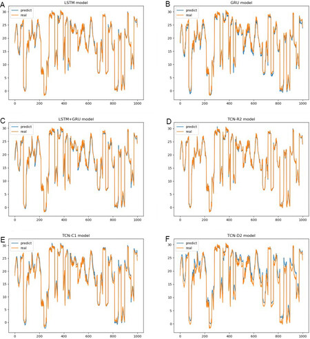
Figure 6. Predictions of several models. LSTM: Long short-term memory; GRU: gated recurrent unit; TCN: temporal convolutional network.
Next, we modified two random temperature data into abnormal data to test the robustness of the LSTM-GRU and TCN-R2. The test results are shown in Figure 7. Furthermore, the EVS and MSE are shown in Table 3.
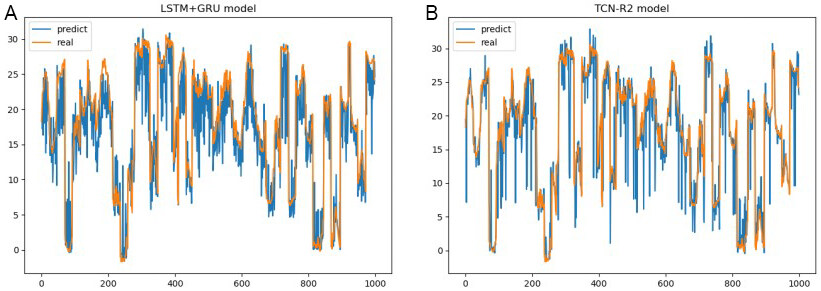
Figure 7. The result of abnormal data on LSTM-GRU and TCN-R2. LSTM: Long short-term memory; GRU: gated recurrent unit; TCN: temporal convolutional network.
The EVC and MSE in abnormal data of the two models.
| EVS | MSE | |
| LSTM-GRU TCN-R2 | 0.8514 0.8247 | 16.1151 15.2085 |
The picture on the left is LSTM-GRU, and the picture on the right is TCN-R2. As shown in Table 3, the EVC of LSTM-GRU is higher, but the MSE is higher than TCN-R2. It shows that the trend value of LSTM-GRU has high accuracy but fluctuates greatly. It can also be confirmed from the results in Figure 7 that LSTM-GRU makes unserious mistakes. Moreover, TCN makes fewer mistakes, but it always predicts great extremes and wrong trends. However, TCN-R2 can produce extreme outliers of more than 30 °C. Therefore, TCN-R2 is not competent in an environment with many invalid sensor data.
5. CONCLUSIONS
In this paper, two kinds of network structures for predicting thermocline time series data are proposed. One is the LSTM-GRU hybrid neural network model, and the other is the TCN-based neural network model. The two networks have obvious advantages over other models in accuracy, stability, and adaptability. TCN has higher prediction accuracy, while LSTM-GRU can better predict abnormal data and has higher robustness. For future work, other variables, such as location blocks and atmospheric parameters, can be added to the model to better predict ocean temperature and improve the accuracy of ocean temperature prediction. This paper only concerns ocean surface temperature. Deep seawater is also a vital topic, and it is more practical to predict the temperature of shallow seawater and deep seawater simultaneously. Forecasting multiple data in different depths adds one dimension to the data, and this will be another challenge as seawater exhibits nonlinear vertical variations.
DECLARATIONS
Authors’ contributions
Made substantial contributions to conception and design of the study: Jiang Y, Zhao M
Performed data analysis and interpretation: Zhao W, Qin H, Qi H
Performed data acquisition, as well as providing, technical, and material support: Wang K, Wang C
Availability of data and materials
The Argo data were collected and made freely available by the International Argo Program and the national programs that contribute to it (http://www.argo.ucsd.edu, http://argo.jcommops.org). The data using in this paper could be found and downloaded from ftp://ftp.argo.org.cn/pub/ARGO/global/.
Financial support and sponsorship
This work was supported by the National Natural Science Foundation of China under Grant 62072211, Grant 51939003, and Grant 51809112.
Conflicts of interest
All authors declared that there are no conflicts of interest.
Ethical approval and consent to participate
Not applicable.
Consent for publication
Not applicable.
Copyright
© The Author(s) 2021.
REFERENCES
1. Zhang Q, Wang H, Dong J, Zhong G, Sun X. Prediction of sea surface temperature using long short-term memory. IEEE Geosci Remote Sensing Lett 2017;14:1745-9.
3. Jiang Y, Zhang T, Gou Y, He L, Bai H, Hu C. High-resolution temperature and salinity model analysis using support vector regression. J Ambient Intell Human Comput 2018; doi: 10.1007/s12652-018-0896-y.
4. Jiang Y, Gou Y, Zhang T, Wang K, Hu C. A machine learning approach to Argo data analysis in a thermocline. Sensors (Basel) 2017;17:2225.
5. Li X, Liang Y, Zhao M, Wang C, Jiang Y. Few-shot learning with generative adversarial networks based on WOA13 data. Computers, Materials & Continua 2019;60:1073-85.
6. Jiang Y, Zhao M, Hu C, He L, Bai H, Wang J. A parallel FP-growth algorithm on World Ocean Atlas data with multi-core CPU. J Supercomput 2019;75:732-45.
7. Xue Y, Leetmaa A. Forecasts of tropical Pacific SST and sea level using a Markov model. Geophys Res Lett 2000;27:2701-4.
8. Landman WA, Mason SJ. Forecasts of near-global sea surface temperatures using canonical correlation analysis. J Climate 2001;14:3819-33.
9. Penland C, Magorian T. Prediction of Niño 3 sea surface temperatures using linear inverse modeling. J Climate 1993;6:1067-76.
10. Johnson SD, Battisti DS, Sarachik ES. Empirically derived markov models and prediction of tropical pacific sea surface temperature anomalies*. J Climate 2000;13:3-17.
11. Tangang FT, Hsieh WW, Tang B. Forecasting the equatorial Pacific sea surface temperatures by neural network models. Climate Dynamics 1997;13:135-47.
12. Mahongo SB, Deo MC. Using artificial neural networks to forecast monthly and seasonal sea surface temperature anomalies in the Western Indian Ocean. The International Journal of Ocean and Climate Systems 2013;4:133-50.
13. Bhaskaran PK, Rajesh Kumar R, Barman R, Muthalagu R. A new approach for deriving temperature and salinity fields in the Indian Ocean using artificial neural networks. J Mar Sci Technol 2010;15:160-75.
14. Xiao C, Chen N, Hu C, Wang K, Gong J, Chen Z. Short and mid-term sea surface temperature prediction using time-series satellite data and LSTM-AdaBoost combination approach. Remote Sensing of Environment 2019;233:111358.
15. Yang Y, Dong J, Sun X, Lima E, Mu Q, Wang X. A CFCC-LSTM model for sea surface temperature prediction. IEEE Geosci Remote Sensing Lett 2018;15:207-11.
16. Box G. Time series analysis, forecasting and control. Rev. ed. San Francisco: Holden-Day; c1976.
17. Zhang G. Time series forecasting using a hybrid ARIMA and neural network model. Neurocomputing 2003;50:159-75.
20. Liu Y, Wang X, Zhai Z, Chen R, Zhang B, Jiang Y. Timely daily activity recognition from headmost sensor events. ISA Trans 2019;94:379-90.
22. Ergen T, Kozat SS. Efficient online learning algorithms based on LSTM neural networks. IEEE Trans Neural Netw Learn Syst 2018;29:3772-83.
23. Gers FA, Schmidhuber J, Cummins F. Learning to forget: continual prediction with LSTM. Neural Comput 2000;12:2451-71.
25. Zhang Z, Pan X, Jiang T, Sui B, Liu C, Sun W. Monthly and quarterly sea surface temperature prediction based on gated recurrent unit neural network. JMSE 2020;8:249.
Cite This Article
Export citation file: BibTeX | RIS
OAE Style
Jiang Y, Zhao M, Zhao W, Qin H, Qi H, Wang K, Wang C. Prediction of sea temperature using temporal convolutional network and LSTM-GRU network. Complex Eng Syst 2021;1:6. http://dx.doi.org/10.20517/ces.2021.03
AMA Style
Jiang Y, Zhao M, Zhao W, Qin H, Qi H, Wang K, Wang C. Prediction of sea temperature using temporal convolutional network and LSTM-GRU network. Complex Engineering Systems. 2021; 1(2): 6. http://dx.doi.org/10.20517/ces.2021.03
Chicago/Turabian Style
Jiang, Yu, Minghao Zhao, Wanting Zhao, Hongde Qin, Hong Qi, Kai Wang, Chong Wang. 2021. "Prediction of sea temperature using temporal convolutional network and LSTM-GRU network" Complex Engineering Systems. 1, no.2: 6. http://dx.doi.org/10.20517/ces.2021.03
ACS Style
Jiang, Y.; Zhao M.; Zhao W.; Qin H.; Qi H.; Wang K.; Wang C. Prediction of sea temperature using temporal convolutional network and LSTM-GRU network. Complex. Eng. Syst. 2021, 1, 6. http://dx.doi.org/10.20517/ces.2021.03
About This Article
Copyright

Data & Comments
Data


 Cite This Article 22 clicks

 Like This Article 4
likes
Like This Article 4
likes


Comments
Comments must be written in English. Spam, offensive content, impersonation, and private information will not be permitted. If any comment is reported and identified as inappropriate content by OAE staff, the comment will be removed without notice. If you have any queries or need any help, please contact us at support@oaepublish.com.