
A qLPV Nonlinear Model Predictive Control with Moving Horizon Estimation

 , ...
, ... Abstract
This paper presents a Model Predictive Control (MPC) algorithm for Nonlinear systems represented through quasi-Linear Parameter Varying (qLPV) embeddings. Input-to-state stability is ensured through parameter-dependent terminal ingredients, computed offline via Linear Matrix Inequalities. The online operation comprises three consecutive Quadratic Programs (QPs) and, thus, is computationally efficient and able to run in real-time for a variety of applications. These QPs stand for the control optimization (MPC) and a Moving-Horizon Estimation (MHE) scheme that predicts the behaviour of the scheduling parameters along the future horizon. The method is practical and simple to implement. Its effectiveness is assessed through a benchmark example (a CSTR system).
Keywords
1. INTRODUCTION
Model Predictive Control (MPC) is a very powerful control method, with widespread industrial application. The core idea of MPC [1] is simple enough: a process model is used to predict the future output response of the process; then, at each instant, the control law is found through the solution of an online optimization problem, which is written in terms of the model, the process constraints and the performance goals. For the case of processes represented by Linear Time-Invariant (LTI) models, MPC is translated as a constrained Quadratic Programming Problem (QP), which can be evaluated in real-time by the majority of standard solvers.
Extra attention should be payed to the fact that the theoretical establishment MPC was especially consolidated after the proposition of “terminal ingredients”, which served to demonstrate robust stability and recursive feasibility properties [2]. These properties are enabled when some conditions with respect to a terminal stage cost V(·) and to a terminal constraint Xf are verified. Essentially, the terminal set must be robust positively invariant for the controlled system, the stage cost must be
For many years, MPC was mostly seen in the process industry, regulating usually slower applications (with longer sampling periods). This was mainly due to the fact that the inherent optimization procedures were excessively costly (numerical-wise) and became impractical for real-time systems.
Nonlinear MPC (NMPC) algorithms yield complex optimization procedure, with exponential growth of the numerical burden. Nevertheless, the majority of system is indeed nonlinear and, thus, literature has devoted special attention to feasible NMPC design since the 00’s [3]. Originally, NMPC algorithms were hardly able to run in real-time [4], but recent research effort has focused to a great extent on ways to simplify or approximate, usually through Gauss-Newton, Lagrangian or multiple-shooting discretization approaches [5], the online Nonlinear Programming Problem (NP) in order to make it viable for fast, time-critical processes. Some of these faster NMPC algorithms run within the range of a few milliseconds, resorting to solver-based solutions (as in ACADO[6] or GRAMPC[7] algorithms) or GPU-based schemes[8,9].
Parallel to these approximated methods, another research route is now expanding to address the complexity drawback of “full-blown” NMPC strategies: using quasi-/Linear Parameter Varying (qLPV/LPV) model structures to embed the nonlinear dynamics, as in [10], and thus facilitate the online optimization. Since LPV models retain linearity properties through the input/output channels, the optimization can be reduced to the complexity of a QP. A recent survey[11] details the vast possibilities of issuing NMPC through LPV structures. The basic requirement of these methods is that the nonlinearities must respect the Linear Differential Inclusion (LDI) property[12,13], in such a way that they can be embedded into a qLPV realisation, appropriately “hidden” in scheduling parameters ρ.
Instead of using a moving-window linearization strategy to yield fast NMPCs with time-varying models[14], or of using approximated solutions of the NP iterations [6], this paper follows the lines of the qLPV embedding framework, which allows for an exact description of the nonlinear system and, thereby, no time-consuming linearization or Jacobian computation needs to take place. As previously evidenced[11], these qLPV methods are able to use the scheduling proxy ρ(k) = f(x(k), u(k)) to compute the process predictions rapidly. In fact, these methods have recently been shown [15] to outrank (or perform equivalently as) fast NMPC solvers, such as ACADO. Some of these recent development are further detailed:
Some works[
16 ,17 ] opt to consider a frozen/constant guess for the scheduling parameters along the future horizon and ensure, through the use of terminal ingredients, that the trajectories are sufficiently regulated, despite the uncertainty along the horizon;Morato et al. [
18 ] propose a method to determine an educated estimation for scheduling variables using a recursive Least-Squares procedure. A similar procedure is applied in[19 ]. The main drawback is that the results could be sub-optimal, meaning that local minima found through their QPs/ Sequential QPs (SQPs), which may not ensure sufficient performances.The most prominent results are those reported in the recent works by Cisneros & Werner [
20 -22 ]. The original idea[20 ] is to iteratively use the prediction for the future state trajectories (output of the QP) to compute a guess of the scheduling parameters, using the nonlinear proxy ρ(k + j) = f(x(k + j)). The method was extended [21 ] to reference-tracking and shown to yield a Second-order Cone Program (2ndOCP) formulation for the resulting NMPC, which is easier to solve than an NP. The formulation was further smoothed in the most novel reference [22 ], wherein the procedure is split into an offline preparation part, using Linear Matrix Inequalities (LMIs) to compute a robust positively invariant terminal set, and an online residing solely in re-iterating SQPs.
1.1. Contributions and rganization
oAs detailed in the prequel, the topic of NMPC through qLPV embedding has been studied by a handful of papers and deserves further attention. It seems that the development of these strategies can surely be established as a competitive category for nonlinear MPC design, regarding time-critical applications.
Pursuing this matter and motivated by the previous discussion, this paper proposes an alternative formulation to the recent algorithm by Cisneros and Werner[22]. In their work, the nonlinear proxy has to be evaluated online w.r.t. to the future state evolution prediction originated through the QP. The alternative procedure proposed herein relies on approximating the nonlinear proxy by a time-varying auto-regressive function, whose parameters are found through another QP, based on a Moving-Horizon Estimation (MHE) method. This alternative is able to slightly boost the numerical performances of the whole algorithm, which only needs to evaluate three QPs to find the control law.
Accordingly, the contributions presented are the following:
An alternative formulation for NMPC is proposed: using qLPV embeddings, the MPC operates together with an MHE layer, which estimates the future behaviour of the scheduling parameters.
The convergence of the algorithm is demonstrated.
A benchmark example is used to demonstrate the effectiveness of the proposed scheme, in terms of performance and numerical burden.
Regarding organization, this paper is structured as follows. Idn the next Section, the preliminaries and formalities are presented, especially regarding how nonlinear processes can be embedded into a qLPV representation through LDI. Moreover, the problem setup regarding MPC applied to such qLPV model is presented. Furthermore, the proposed MHE-MPC formulation and the discussion about stability and an offline LMI-solvable remedy for the computation of the terminal ingredients is addressed. Lastly, Section simulation results and general conclusions are drawn.
1.2. Basic efinitions
Definition 1. Nonlinear Programming Problem
Consider an arbitrary real-valued nonlinear function fc(xc). A Nonlinear Programming Problem determines the vector xc that minimizes fc(xc) subject to gi(xc) ≤ 0, hj(xc) = 0 and
Definition 2. Quadratic Programming Problem
A Quadratic Programming Problem (or simply Quadratic Problem) is a linearly constrained mathematical optimization problem of a quadratic function. A QP is a particular type of NP. The quadratic function may be defined with respect to several variables, all of which may be subject to linear constraints. Considering a vector
1.3. Notation
In this work, the set of non-negative real number is denoted by
The value of a given variable v(k) at time instant k + i, computed based on the information available at instant k, is denoted as v(k + i\k).
Finally, consider two sets
2. PRELIMINARIES
In this Section, we detail how nonlinear processes can be described under a qLPV formalism; we also present some other formalities.
2.1. The Nonlinear System and its qLPV Embedding
We consider the following generic discrete-time nonlinear system:
where
We begin by characterizing this process, which should satisfy the following key Assumptions:
Assumption 1.The admissible zone for the states is given by a 2-norm upper bound on each entry xj, this is:
Assumption 2.The admissible region for the control inputs is given by a 2-norm upper bound on each entry uj, this is:
Assumption 3.The nonlinear maps
Assumption 4.This nonlinear system is controllable in terms of x and y through the input trajectory u.
To represent any nonlinear system, as the one in Eq. (1), under a qLPV formalism, this last Assumption must be verified, since it is the LDI property that furnishes the settings for such representation.
The LDI property is as follows: suppose that, for each x, u and y and for every sampling instant k, there exists a matrix
where
which is a qLPV formulation where
We consider that the qLPV scheduling parameters have bounded rates of variations, this is: ρ(k + 1) = ρ(k) + ∂ρ(k + 1), being
3. PROBLEM SETUP
Regarding the qLPV embedded model in Eq. (5), we proceed by detailing how MPC can be applied to regulate and control this system. For the simplify of the reference tracking demonstrations, we drop the input-output energy transfer, i.e. D(ρ(k)) = 0. We note that the processes with D(ρ(k)) ≠ 0 can still be dealt with the proposed method, we no additional drawbacks.
The essential idea behind MPC is to consider a quadratic finite-horizon functional cost, which embeds the performance objectives of the system within this given horizon. The implementation resides in minimizing this cost with respect to a control signal sequence, using a model of the system in order to make predictions for the future variable values along the horizon. The optimization also includes the operational constraints of the process variables (admissibility region). Generically, we consider the following steady-state reference tracking performance cost:
where Q and R are positive definite weighting matrices and the pair (xr, ur) defines a known admissible steady-state reference target for the nonlinear system. The optimization cost J considers a prediction horizon of Np steps and a positive terminal stage value V (x(k + Np|k)) > 0.
The MPC framework considers a moving-window strategy. Therefore, at each sampling instant k, since x(k), and ρ(k) are known, the corresponding optimization problem is solved, which gives the solution
whose first input u(k|k) = I1Uk is applied to the process. Then, the horizon slides forward and the procedure is updated. The complete optimization, at each sampling instant k, is given as follows:
where Xf and V(·) are the terminal ingredients, combined to ensure recursive feasibility of the algorithm (see Section Stability and Offline Preparations).
Due to Eq. (8), it follows that the future values for the qLPV scheduling variables ρ(k + i) are not known for any i ≥ 1. At each instant k, the optimization operates based on the knowledge of x(k) and u(k), which can be used to compute ρ(k) through the nonlinear qLPV proxy fρ(·). One could easily include this proxy into the optimization, making it also subject to ρ(k + i) = fρ (x(k + i), u(k + i)) together with the process model, but this would convert Eq. (8) into a Nonlinear Programming Problem, which is associated with numerical complexity issues (as previously discussed).
The NP execution is computationally unattractive[22] because of this general nonlinear dependence of the predicted states on the control inputs and on previous states. Therefore, following the lines of previous works [19,22], this paper pursues a fast implementation of the LPV MPC optimization procedure in Eq. (8), which means that we do not seek to analytically include the nonlinear qLPV scheduling proxy fρ (·) to the optimization, but rather to provide values for the complete evolution of the scheduling parameters along the prediction horizon, as if they were known (thus detaching the nonlinear dependency). This is, we aim to solve Eq. (8) based on x(k), ρ(k) and on the future ”scheduling sequence” vector
If the actual evolution of the scheduling sequence is as gives Pk, the MPC ensures perfect regulation. Furthermore, it is formulated as a Quadratic Programming Problem, which can be tackled for many time-critical applications with modern solvers. In fact, we approximate the NP solution by one which resides in a ”guess” for the scheduling sequence Pk, which attractively converges to the actual value of this vector as the procedure iterates. The solution to estimate Pk is based on a Moving Horizon Estimation algorithm, which is further detailed in Section The MHE-MPC Mechanism.
We must proceed by providing some complementary Assumptions regarding this qLPV MPC optimization problem setup. For such, we denote
Assumption 5.The qLPV scheduling proxy is set-wise and vector-wise applicable, this is, it holds as
Assumption 6.The application of the scheduling proxy to the admissible zone for the states and inputs is a subset of the scheduling set, this is:
Assumption 7.The admissible region
From the viewpoint of each sampling instant k, the scheduling sequence can be directly evaluated as:
where
which is directly given by
With the previous discussion in mind, we proceed by using the qLPV model from Eq. (5) and the definitions from Eqs. (7), (9) and (10) to analytically provide a solution to the state evolution which is explicitly dependent on the scheduling sequence.
For the LTI case, the state evolution Xk, departing from x(k), is expressed on a linear dependent basis w.r.t. x(k) and to the sequence of control inputs Uk, as follows:
Analogously, for the qLPV case, since linearity is retained through the input-output channels (i.e. from u to x), the state evolution can be given in a quite similar fashion, but with parameter dependence on Pk appearing on the transition matrices, this is:
where the parameter dependent matrices are given by [
In order to compute matrices
where H(Pk) is the Hessian of this cost function, g(·) its gradient and κ(·) an offset term. The notation Q̆ and R̆ denote the block-diagonal version of these matrices, i.e.
3.1. Process constraints
The qLPV MPC problem solution proposed in this paper is formulated with respect to the scheduled state evolution equation, as gave Eq. (15), with H(Pk), g(·) and κ(·) being as passed as inputs to the resulting MPC optimization. This means that the MPC optimization does not treat state evolution Xk as optimization variables, but the whole problem is formulated singularly in terms of Uk.
For this reason, the admissibility process constraints
The above formulations also facilitates the inclusion of slew rates on u, i.e. constraints on the control variation δu(k + i) = u(k + i) – u(k + i – 1), which can be done directly by adapting the vector-wise set
The terminal constraint x(k + Np|k) ∈ Xf is stated in terms of Uk as:
where
Additional output constraints are also easily formulated. If the process has some outputs yc (which are not necessarily equal to y, but could be) that must be hard constrained, i.e.
In what follows, we take
Then, the additional constraint is formulated as follows [Note that the last
thus
3.2. Reference tracking
Finally, before showing the proposed mechanism to guess Pk and solve the qLPV MPC problem, a comment must be made regarding reference tracking. The considered cost function J(x, u, k) from Eq. (6) (or its vector form of Eq. (16)) is set in order to minimize the variations from the desired set-point target pr= (xr, ur).
The majority of processes that require reference tracking, require it regarding the controlled outputs and not the states. This is, to ensure that y(k) tracks some steady-state value yr. Since the controlled outputs in Eq. (5) are given by
we can find a linear (parameter varying) combination of the states x that, if tracked, ensures that y(k) → yr. We denote the output tracking target as
Then, following the lines of previous reference tracking frameworks [24-26], we use an offline reference optimization selector, which is set to find the set-point target pr that abides to the constraints and ensures an output tracking of yr. This nonlinear optimization procedure is as follows:
This procedure ensures some steady-state xr= A(ρr)xr + B(ρr)ur ) that abides to the states constraints and guarantees that the output tracking goal yr is followed.
Note that this optimization procedure has a steady-state target point pr= (xr, ur) as output, and not the full state and input trajectories towards this target.
The state reference selection problem can be solved online, at each sampling instant, if the output reference goal yr changes over time. By doing so, an additional computational complexity appears, which can be smoothed if the scheduling parameter guess Pk is used instead of solving the nonlinear optimization itself. A full discussion on periodically changing reference tracking for nonlinear MPC has been recently presented [27]. The focus of this paper is constant reference signals, either given in terms of states xr or outputs yr
It is important to notice that, in order for the method to hold, the state reference xr must be contained inside the terminal set of the MPC problem from Eq. (8). This ensures that the stability and recursive feasibility guarantees (as verified in Section Stability and Offline Preparations) hold.
4. THE MHE-MPC MECHANISM
In the general qLPV embedding case of Eq. (5), the scheduling proxy fρ(·) is an arbitrary function of both state and input. For notation ease, we drop the control input dependency, using taking ρ(k) = fρ(x(k)). Anyhow, note that all that follows can be trivially extended to broader case.
The backbone idea of the method proposed in this paper follows the fashion of previous papers[19,22]: to iteratively refine the predictions/guesses of the scheduling sequence Pk based on the (adjusted) state predictions
A priori, the operation of this MHE has the computational complexity of a QP, which could be faster to evaluate than the Eqs. (13) with
Assumption 8.The scheduling map fρ(·) is algebraic.
Proposition 1.The scheduling map
which can be given in compact form by:
being
Proof. Indeed, due to Assumption 8, it is quite reasonable that Assumption 1 holds: any algebraic function of form ρ(k + 1) = fρ(x(k + 1)) can be Taylor-expanded to achieve a linear dependency on x with sufficiently small error, i.e.
This concludes the proof. □
The proposed procedure uses a MHE mechanism to estimate these parameter values a0,0 to aNp–1,Np–1-1, at each sampling instant, concatenated as Θk,through the following QP:
Essentially, this MHE scheme operates in order to find a parameter matrix Θk that makes the linear auto-regressive equation
Figure 1 syntheses the proposed algorithm, which relies in a coordination between the MHE and the MPC optimization procedures. We must note that the MHE loop should operate until Pk converges to the actual value for the scheduling sequence, or until a certain stop criterion/heuristic threshold for the number of iterations is reached.
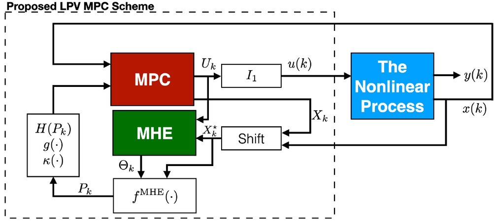
Figure 1. Proposed MHE-MPC Scheme using a qLPV Model.
The proposed scheme is also detailed through the Algorithm below. Its application departs with an initial state evolution sequence X0, that can be simply taken as constant/frozen evolution for the states and two initial scheduling sequences P0 and P–1, which can be simply taken as if ρ(k) remained frozen along the whole prediction horizon, i.e.
4.1. Convergence property
In order to demonstrate the convergence of the proposed method (as in its implementation form given in Algorithm 1), we will proceed by verifying a well-known results for Newton based SQPs from the literature [28-30]. This is the same path followed in a previous paper [22], which invokes established results to demonstrate that, under certain conditions, the MHE-MPC mechanism that is solved at each iteration is equivalent to a quadratic sub-problem used in standard Newton SQP. Therefore, a local convergence property is readily found.
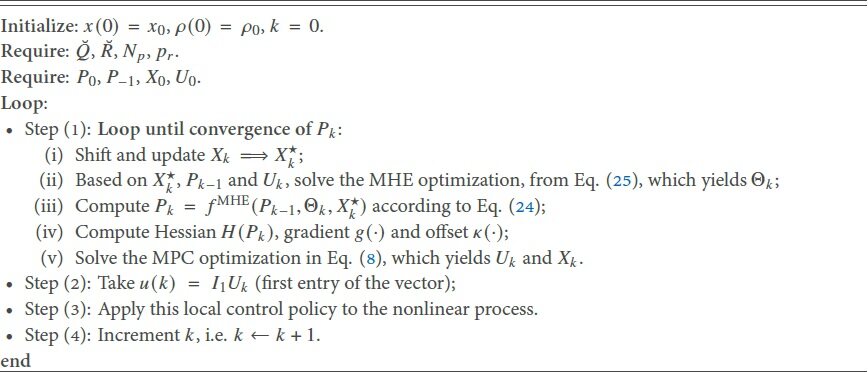
Algorithm 1. Proposed qLPV MPC
Proposition 2.A quadratic sub-problem program of SQP algorithms is derived by a second-order approximation of the SQP optimization cost and a linearization of its constraints.
Proof. Found in [28]. □
For illustration purposes regarding this matter, we consider the following generic NP (as given in Definition 1):
This problem can be given as a quadratic sub-problem directly, as follows:
where Hfc (xc) denotes the Hessian of the optimization cost fc(xc) and ∇hj(xc) and ∇gi(xc) denote divergent operators. We note that this sub-problem is evaluated at a given solution estimate x̅c (at some given iteration), for which
Regarding the proposed MHE-MPC mechanism, we can easily show that if either simple Jacobian linearization or Linear Differential Inclusion are used to find a qLPV model (as in Eq. (5)) for the nonlinear system (as in Eq. (1)), then, the proposed mechanism iterates in equivalence to a Newton SQP sub-problem. Notice how such sub-problem in Eq. (27) is identical to the MHE-MPC optimization given through the consecutive iterations of the MHE (Eq. (25)) and the MPC (Eq. (8)). The terminal constraint in the MPC optimization adds no convergence trade-off.
Thence, it follows that if local convergence of the equivalent Newton SQP can be established, the proposed MHE-MPC also yields convergence. The sufficient conditions for local convergence of a Newton SQP sub-problem at xc =x̅c, as given by prior references [29-32], are that (i) the problem is set simply with equality constraints (not the MPC case) or that (ii) the subset of active inequality constraints are known before the optimization solution. The second condition is also not true for general MPC paradigms. However, one can iterate the sub-problem until convergence is found at another point
In practice, the proposed MHE-MPC will not be set to freely iterate until the convergence of Pk. This is not desirable because the number of iterations needed for convergence may require more time than the available sampling period. Therefore, a stop criterion is added to the mechanism, so that iterations stop at a given threshold. A warm-start is also included by shifting the result regarding Xk and Pk from one sampling k as the initial guess for the optimization at k + 1, which ensures that the proposed algorithm reaches convergence after a few discrete-time samples. We note that convergence of Newton SQP sub-problems with warm-start have been assessed [33,34] and shown to be practicable for real-time schemes.
5. STABILITY AND OFFLINE PREPARATIONS
In this Section, we offer a Theorem to construct the terminal ingredients of the MPC algorithm: (a) the terminal set within which x(k + Np|k) is bounded to, and (b) the terminal offset cost V(x(k + Np|k)) minimized by the MPC.
Since the establishment of terminal ingredients toolkit [2,35] as the key way to ensure stability and recursive feasibility of state-feedback predictive control loops, MPC grew on both theory and industrial practice.
The usual approach with terminal ingredients resides in some ensuring that conditions are met by (a) the terminal set Xf and (b) the terminal cost V(x(k + Np|k)) with respect to a nominal state-feedback controller u(k) = knx(k), which is usually the unconstrained solution of the MPC problem. For the tracking case, the nominal feedback is given by u(k) = kn (x(k) – xr) (and so is the terminal constraint (x(k + Np|k) – xr) ∈ Xf and the terminal cost V(x(k + Np|k) – xr)). Accordingly we develop a sufficient stability condition for the proposed MHE-MPC mechanism in order to verify these conditions.
Firstly we consider that there exists a parameter-dependent nominal state-feedback gain
This nominal controller is purely fictional, used to demonstrate stability and recursive feasibility properties of the proposed MHE-MPC mechanism. Anyhow, it stands for the infinite-horizon LPV Linear Quadratic Regulator (LQR) solution, which verifies
Of course, there is a complexity barrier to solve this problem, because the states have parametric nonlinearities that impact their trajectories (the qLPV scheduling parameters). Therefore, we determine this nominal feedback gain together with the terminal ingredients, which are also taken as parameter-dependent on ρ. We consider, for regularity, an ellipsoidal set as the terminal constraint, which is given by:
This ellipsoid is centered at the origin and has a radius of αp. Furthermore, this terminal set is a sub-level set of terminal cost V(·), which is taken as a Lyapunov function as follows:
This parameter-dependent nominal feedback gain Kn(ρ)) and the parameter dependent terminal ingredients verbalized through the symmetric parameter dependent Lyapunov matrix P(ρ) are so that the following input-to-state stability Theorem is guaranteed.
Theorem 1.Input-to-State Stable MPC[2,22,35,36]
Let Assumptions 4 and 7 hold. Assume that a nominal control law u = Kn(ρ)x exists. Consider that the MPC is in the framework of the optimization problem in Eq. (8), with a terminal state set given by Xf(ρ) and a terminal cost V(x,ρ). Then, input-to-state stability is ensured if the following conditions are hold
(C1) The origin lies in the interior of Xf(ρ);
(C2) Any consecutive state to x, given by (A(ρ) + B(ρ)Kn(ρ)) x lies withinXf(ρ) (i.e. this is an invariant set);
(C3) The discrete algebraic Ricatti equation is verified within this invariant set, this is, ∀ x ∈ Xf (ρ(k)):
$$ \begin{align*} V((A(\rho(k))+B(\rho(k)) K^{n}(\rho(k))) x, \rho(k+1))-V(x, \rho(k)) \\ \leq-x^{T} Q x-x^{T}\left(K^{n}(\rho(k))\right)^{T} R K^{n}(\rho(k)) x . \end{align*} $$ (C4) The image of the nominal feedback always lies within the admissible control input domain:
. (C5) The terminal set Xf (ρ) is a subset of the admissible state domain
$$ \mathcal{X} $$
Assuming that the initial solution of the MPC problem
Proof. Provided in Appendix Proof of Theorem 1. □
In order to find some nominal state-feedback gain Kn(ρ), some terminal set Xf and some terminal offset cost V(·), an offline LMI problem is proposed in the sequel. This LMI problem is such that a P(ρ) positive definite parameter-dependent matrix is found to ensure that the conditions of Theorem 1 are satisfied. Due to condition (C3), the LMI is solved over a sufficiently dense grid over ρ, consider its admissibility domain
This LMI problem is provided through the following Theorem, which aims to find the largest terminal set Xf that is invariant under the nominal control policy u(k) = Kn(ρ(k))x(k) for all k, while remaining admissible, i.e.
Theorem 2.Terminal Ingredients[22,37]
The conditions (C1)-(C5) of Theorem 1 are satisfied if there exist a symmetric parameter-dependent positive definite matrix
where Ij denotes the j-throw of the identity matrix
Proof. Refer to[37]. □
We must note that the above proof demonstrates that the solution of the LMIs presented in Theorem 2 ensure a positive definite parameter dependent matrix P(ρ) which can be used to compute the MPC terminal ingredients V(·) and Xf such that input-to-state stability of the closed-loop in guaranteed, verifying the conditions of Theorem 1. Furthermore, when the MPC is designed with these terminal ingredients, for whichever initial condition x(0) ∈ Xf it starts with, it remains recursively feasible for all consecutive discrete time instants k > 0.
Anyhow, Theorem 2 provides infinite-dimensional LMIs, since they should hold for all
6. BENCHMARK EXAMPLE
In this Section, we pursue the application of the proposed MHE-MPC mechanism with terminal ingredients found through Theorem 2. For such, we consider the application of our control method upon a benchmark system, detailed in the sequel.
6.1. Continuously-stirred tank reactor
Consider the model of a Continuously-Stirred Tank Reactor (CSTR) process, which consists of an irreversible, exothermic reaction, A → B, in a constant volume reactor cooled by a single coolant stream which can be modeled by the following equations:
where CA is the concentration of A in the reactor, T is the temperature in the reactor, and Tc is the coolant temperature.
In this process, u = Tc is a control input, whereas CA and T are measurable process variables. The considered model parameters and process constraints are reported in Table 1.
Model Parameters and Constraints
| Parameter | Value/Set | Parameter | Value/Set |
|---|---|---|---|
| q | 100 L min–1 | CAf | 1 mol L–1 |
| k0 | 7.2 × 10¹⁰ min–1 | E/R | 8750 K |
| HΔ | –5 × 10⁵ cal mol–1 | ρCp | 239 cal L–1 K–1 |
| W | 7 × 5104 cal min–1 K–1 | V | 100 L |
| Tf | 350K | - | - |
| CA | ∈ [0.03, 0.12] mol 1–1 | T | ∈[440,460] K |
| Tc | ∈ [200, 380]K | - | - |
6.2. qLPV Embedding
Considering x = (CA, T) as state variables, we obtain the following qLPV realization of the CSTR system from Eq. (33):
where ρ = f(x) denotes two scheduling variables, given as linear functions of each state, i.e. ρ1= f1(x1) and ρ2=f2(x2). This continuous-time model is Euler-discretized using a sampling period of Ts= 30ms.
6.3. Control goal and tuning
Considering an arbitrary initial condition x0 given within the state admissibility set
The MHE scheme, which is used to estimate the future scheduling behaviour Pk at each sampling instant k, is set to operate with a threshold loop barrier of 3 loops, which is a verified sufficient bound to induce convergence (refer to the discussion in Section Convergence Property).
6.4. Simulation results
Considering a realistic nonlinear CSTR model, we obtain simulation results to demonstrate the effectiveness of the proposed control scheme. The following results were obtained in a 2.4 GHz, 8 GB RAM Macintosh computer, using Matlab, yalmip and Gurobi solver.
First, we show how the MHE operation is able to accurately predict the behaviour of the scheduling trajectory, as depicts Figure 2. At each instant k, the MHE provides estimation for Pk, which is composed of the following Np entries of the scheduling variables. In this Figure, we observe the real scheduling variables ρ1 and ρ2 (dot-dash black line) and the estimates Pk provided at different samples (coloured x-marked lines). Within some samples, we can see that the predicted trajectory converges to the real one, which confirms the effectiveness of the MHE operation.
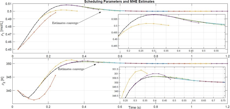
Figure 2. MHE: scheduling trajectory estimates.
Based on the scheduling behaviours predicted by the MHE loop, the predictive controller determines the control input (Figure 4) in order to drive the system states from x0 to the reference goal xr. The corresponding state trajectories are depicted in Figure 3, which also shows the state admissibility set and the terminal set
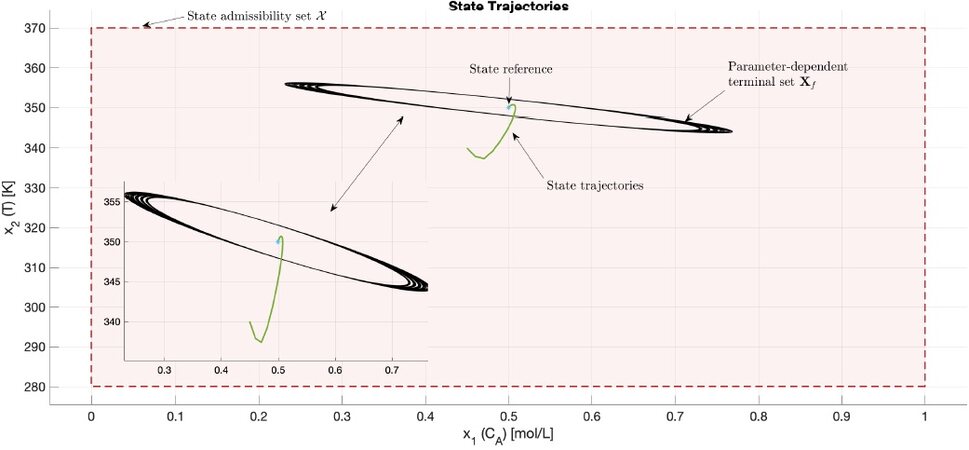
Figure 3. State trajectories, state admissibility set, terminal set.
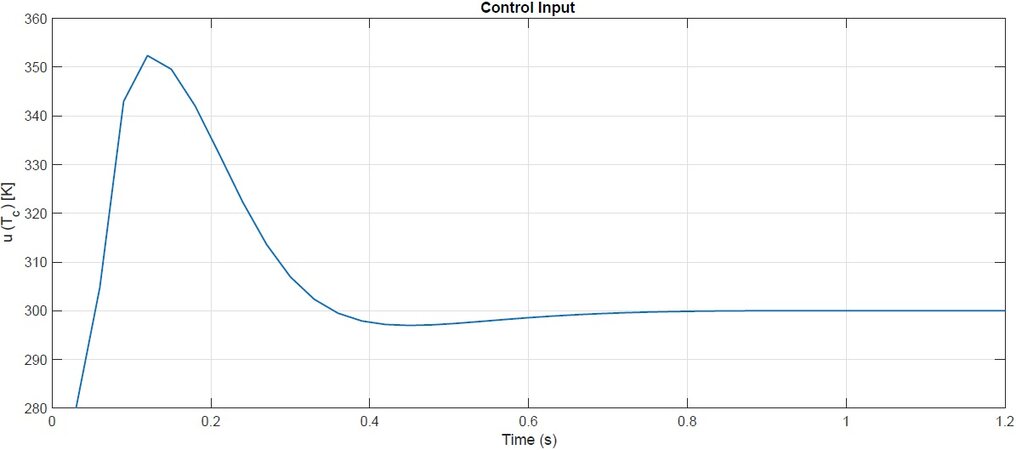
Figure 4. MPC: control input.
Finally, we demonstrate the dissipating properties of the proposed control scheme. In Figure 5, we show the evolution of MPC stage cost J over time. As expected, J decays and converges to the origin, which verifies the dissipation properties required by Theorem 1.
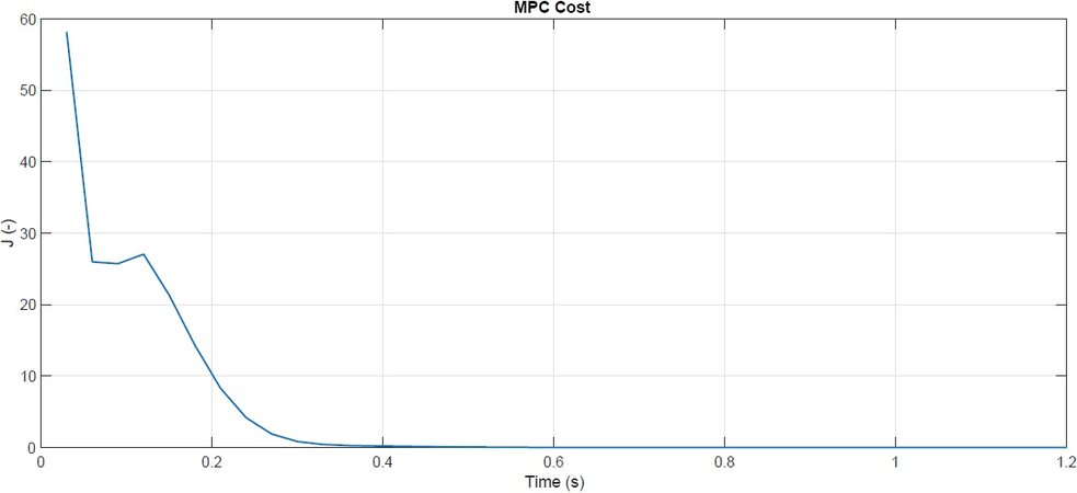
Figure 5. MPC: stage cost.
7. CONCLUSIONS
In this paper, a new method for the fast, real-time implementation of Nonlinear Model Predictive Control is proposed. The method provides a near-optimal, approximated solution, which is found through the online operation of sequential Quadratic Programming Problems. The main necessary argument to develop the method is that the nonlinear process should be described by quasi-Linear Parameter Varying model, for which the embedding is ensured through a scheduling proxy. Then, the online operations resides in the consecutive operation of the MPC program together with a Moving-Horizon Estimation scheme, which is used to match the future values of the scheduling proxy along the prediction horizon, which are unknown. Input-to-state stability and recursive feasibility properties of the algorithm are ensured by parameter-dependent terminal ingredients, which are computed offline. Using a benchmark example, the method is tested. We highlight that it proves itself more effective for stronger nonlinearities in the qLPV scheduling proxy, for which the MHE scheme operates faster than the application of the scheduling proxy upon each entry of the future state variables, as in many other techniques. For future works, the Authors plan on assessing the issue of periodically-changing (possibly unreachable) output reference signals.
DECLARATIONS
Authors’ contributions
All authors contributed equally.
Availability of data and materials
Data will be made available upon e-mail request to the corresponding author.
Financial support and sponsorship
M. M. Morato is partially supported by CNPq project 304032/2019 – 0. V. Stojanovic thanks the Serbian Ministry of Education, Science and Technological Development for support (grant No. 451-03-9/2021-14/200108).
Conflict of interest
Both Authors declare no potential conflict of interests.
Ethical approval and consent to participate
Not applicable.
Consent for publication
Not applicable.
Copyright
© The Author(s) 2021.
REFERENCES
1. Camacho EF, Bordons C. Model predictive control. Springer Science & Business Media; 2013.
2. Mayne DQ, Rawlings JB, Rao CV, Scokaert POM. Constrained model predictive control: Stability and optimality. Automatica, 2000;36:789-814.
3. Allgöwer F, Zheng A. Nonlinear model predictive control, volume 26. Birkhäuser; 2012.
4. Camacho EF, Bordons C. Nonlinear model predictive control: An introductory review. In Assessment and future directions of nonlinear model predictive control. Springer; 2007. pp. 1-16.
5. Gros S, Zanon M, Quirynen R, Bemporad A, Diehl M. From linear to nonlinear MPC: bridging the gap via the real-time iteration. International Journal of Control 2020;93:62-80.
6. Quirynen R, Vukov M, Zanon M, Diehl M. Autogenerating microsecond solvers for nonlinear MPC: a tutorial using ACADO integrators. Optimal Control Applications and Methods 2015;36:685-704.
7. Englert T, Völz A, Mesmer F, Rhein S, Graichen K. A software framework for embedded nonlinear model predictive control using a gradient-based augmented lagrangian approach (GRAMPC). Optimization and Engineering 2019;20:769-809.
8. Ohyama S, Date H. Parallelized nonlinear model predictive control on GPU. In 11th Asian Control Conference, pages 1620–1625. IEEE; 2017.
9. Rathai KMM, Sename O, Alamir M. GPU-based parameterized nmpc scheme for control of half car vehicle with semi-active suspension system. IEEE Control Systems Letters 2019;3:631-6.
10. Hoffmann C, Werner H. A survey of linear parameter-varying control applications validated by experiments or high- fidelity simulations. IEEE Transactions on Control Systems Technology 2014;23:416-33.
11. Morato MM, Normey-Rico JE, Sename O. Model predictive control design for linear parameter varying systems: A survey. Annual Reviews in Control 2020;49:64-80.
12. Boyd S, El Ghaoui L, Feron E, Balakrishnan V. Linear matrix inequalities in system and control theory, volume 15. Siam; 1994.
13. Abbas HS, Toth R, Petreczky M, Meskin N, Mohammadpour J. Embedding of nonlinear systems in a linear parameter-varying representation. IFAC Proceedings Volumes 2014;47:6907-13.
14. Kunz K, Huck SM, Summers TH. Fast model predictive control of miniature helicopters. In 2013 European Control Conference (ECC), pages 1377–1382. IEEE; 2013.
15. Cisneros Pablo SG, Werner Herbert. Wide range stabilization of a pendubot using quasi-LPV predictive control. IFAC-PapersOnLine 2019;52:164-9.
16. Alcalá E, Puig V, Quevedo J. LPV-MPC control for autonomous vehicles. IFAC-PapersOnLine 2019;52:106-13.
17. Mate S, Kodamana H, Bhartiya S, Nataraj PSV. A stabilizing sub-optimal model predictive control for quasi-linear parameter varying systems. IEEE Control Systems Letters 2019; doi: 10.1109/LCSYS.2019.2937921.
18. Morato MM, Normey-Rico JE, Sename O. Novel qLPV MPC design with least-squares scheduling prediction. IFAC-PapersOnLine 2019;52:158-63.
19. Morato MM, Normey-Rico JE, Sename O. Sub-optimal recursively feasible linear parameter-varying predictive algorithm for semi-active suspension control. IET Control Theory & Applications 2020;14:2764-75.
20. Cisneros PSG, Voss S, Werner H. Efficient nonlinear model predictive control via quasi-LPV representation. In IEEE Conference on Decision and Control IEEE; 2016. pp. 3216-21.
21. Cisneros PG, Werner H. Fast nonlinear MPC for reference tracking subject to nonlinear constraints via quasi-LPV representations. IFAC-PapersOnLine 2017;50:11601-6.
22. Cisneros PS, Werner H. Nonlinear model predictive control for models in quasi-linear parameter varying form. International Journal of Robust and Nonlinear Control 2020; doi: 10.1002/rnc.4973.
23. Jungers M, Caun RP, Oliveira RCLF, Peres PLD. Model predictive control for linear parameter varying systems using path-dependent lyapunov functions. IFAC Proceedings Volumes 2009;42:97-102.
24. Limon D, Ferramosca A, Alvarado I, Alamo T, Camacho EF. MPC for tracking of constrained nonlinear systems. In Nonlinear model predictive control Springer; 2009. pp. 315-23.
25. Limon D, Ferramosca A, Alvarado I, Alamo T. Nonlinear MPC for tracking piece-wise constant reference signals. IEEE Transactions on Automatic Control 2018;63:3735-50.
27. Köhler J, Müller MA, Allgöwer F. A nonlinear tracking model predictive control scheme for dynamic target signals. Automatica 2020;118:109030.
28. Qi L. Superlinearly convergent approximate newton methods for lc1 optimization problems. Mathematical programming 1994;64:277-94.
29. Wei Z, Liu L, Yao S. The superlinear convergence of a new quasi-newton-sqp method for constrained optimization. Applied mathematics and computation 2008;196:791-801.
30. Izmailov AF, Solodov MV. On attraction of linearly constrained lagrangian methods and of stabilized and quasi-newton sqp methods to critical multipliers. Mathematical programming 2011;126:231-57.
31. Boggs PT, Tolle JW, Kearsley AJ. On the convergence of a trust region SQP algorithm for nonlinearly constrained optimization problems. In System Modelling and Optimization Springer; 1996. pp. 3-12.
32. Boggs PT, Tolle JW. Sequential quadratic programming for large-scale nonlinear optimization. Journal of computational and applied mathematics 2000;124:123-137.
33. Diehl M, Bock HG, Schlöder JP. A real-time iteration scheme for nonlinear optimization in optimal feedback control. SIAM Journal on control and optimization 2005;43:1714-36.
34. Houska B, Ferreau HJ, Diehl M. An auto-generated real-time iteration algorithm for nonlinear MPC in the microsecond range. Automatica 2011;47:2279-85.
35. Michalska H, Mayne DQ. Robust receding horizon control of constrained nonlinear systems. IEEE transactions on automatic control 1993;38:1623-33.
36. Duan GR, Yu HH. LMIs in control systems: analysis, design and applications. CRC press; 2013.
37. Morato MM, Normey-Rico J, Sename O. Short-sighted robust lpv model predictive control: Application to semi-active suspension systems. In European Control Conference 2021 (ECC21), pages 1–7 2021.
38. Wu F. A generalized LPV system analysis and control synthesis framework. International Journal of Control 2001;74:745-59.
39. Chen H, Kremling A, Allgöwer F. Nonlinear predictive control of a benchmark CSTR. In Proceedings of 3rd European control conference, pages 3247–3252 1995.
Cite This Article
Export citation file: BibTeX | RIS
OAE Style
Morato MM, Bernardi E, Stojanovic V. A qLPV Nonlinear Model Predictive Control with Moving Horizon Estimation. Complex Eng Syst 2021;1:5. http://dx.doi.org/10.20517/ces.2021.09
AMA Style
Morato MM, Bernardi E, Stojanovic V. A qLPV Nonlinear Model Predictive Control with Moving Horizon Estimation. Complex Engineering Systems. 2021; 1(1): 5. http://dx.doi.org/10.20517/ces.2021.09
Chicago/Turabian Style
Morato, Marcelo Menezes, Emanuel Bernardi, Vladimir Stojanovic. 2021. "A qLPV Nonlinear Model Predictive Control with Moving Horizon Estimation" Complex Engineering Systems. 1, no.1: 5. http://dx.doi.org/10.20517/ces.2021.09
ACS Style
Morato, MM.; Bernardi E.; Stojanovic V. A qLPV Nonlinear Model Predictive Control with Moving Horizon Estimation. Complex. Eng. Syst. 2021, 1, 5. http://dx.doi.org/10.20517/ces.2021.09
About This Article
Copyright

Data & Comments
Data


 Cite This Article 31 clicks

 Like This Article 31
likes
Like This Article 31
likes


Comments
Comments must be written in English. Spam, offensive content, impersonation, and private information will not be permitted. If any comment is reported and identified as inappropriate content by OAE staff, the comment will be removed without notice. If you have any queries or need any help, please contact us at support@oaepublish.com.