Research on federated learning method for fault diagnosis in multiple working conditions

1. INTRODUCTION

As an indispensable core component in the connection and transmission chain of mechanical equipment, rolling bearings play an important role in aerospace, electric power, metallurgy, and other industrial fields^[1]. Mechanical equipment working in a complex environment is prone to a higher fault rate related to rolling bearings. Thus, the fault diagnosis of rolling bearings is significant. During the working process of mechanical equipment, the change of load is inevitable, and the change of load will cause the change of the motor speed, which can be seen in the collected data containing vibration data of different loads. Therefore, the fault diagnosis under multiple working conditions is of much practical significance.

In recent years, various methods for fault diagnosis of rolling bearings have been emerged. Data-driven fault diagnosis methods do not require precise physical models and expert knowledge, and they can directly extract data features for fault diagnosis. Therefore, data-driven fault diagnosis methods have attracted much attention from experts in the field of fault diagnosis^[2-3].

Deep learning is a data-driven fault diagnosis method. According to the variance of network structure, it can be classified into four categories: convolutional neural network (CNN)-based methods, long short-term memory network (LSTM)-based methods, deep neural network (DNN)-based methods, and DBN-based methods^[4-7]. DNN and its variations have become some of the most commonly used methods for bearing fault diagnosis due to their simple structure and advantages in processing sequence data. Kong et al.^[8] designed a feature fusion layer to fuse different types of features extracted by DNNs with different activation functions. Liu et al.^[9] performed a short-time Fourier transform on the sound signal of the rolling bearing to generate a spectrogram, and DNN was used to extract features involved in spectrogram. This improved the fault diagnosis capability of the model. Shao et al.^[10] used DAE to extract low-level features from raw vibration signals polluted with Gaussian noise, and then used SDAE to extract high-level features from low-level features to improve fault diagnosis performance. Although the above-mentioned deep learning fault diagnosis method can achieve satisfactory fault diagnosis results, it does not take the situation of multiple working conditions into account.

Due to changes in the external environment, load variation, etc., bearings usually operate under different working conditions in the sense that their process characteristics are quite different; the statistical distribution of the data collected from each working condition are also significantly distinguishable, which violates the constraint of independent and identical distribution required by traditional deep learning algorithms. At present, statistical methods, variational mode decomposition, and decision tree methods are often used to accomplish fault diagnosis under multiple working conditions^[11-13]. Sun et al.^[11] first used PCA to reduce the dimensionality of the data, and then constructed a decision tree to implement a multi-sensor-based multi-condition fault diagnosis method. Song et al.^[12] used a recursive local outlier factor algorithm for adaptive pattern recognition to obtain the principal components according to the cumulative data contribution rate, and the analyzed the critical components that were obtained. The above-mentioned method requires the design of a feature extractor, requires professional knowledge to perform data processing on the collected data signal, and the real-time performance of fault diagnosis cannot be guaranteed.

Existing fault diagnosis methods based on deep learning cannot effectively extract features from multi-working condition data. Therefore, some researchers first classify the working conditions, and then perform fault diagnosis under the situation of multiple working conditions. Zhou et al.^[14] established the DNN model separately for each working condition’s data, which can realize the fault diagnosis of multiple working conditions. Chen et al.^[15] proposed a hierarchical fault diagnosis method based on CNN. The first layer performs working condition recognition and the second layer performs fault type diagnosis. The above-mentioned fault diagnosis methods have high requirements for the accuracy of working condition division, and the result of fault diagnosis is dependent on the efficiency of the working condition division. On the other hand, some scholars use data preprocessing techniques to eliminate modal differences between data and then perform fault diagnosis. Gu et al.^[16] used local nearest-neighbor standardization to eliminate the differences between multimodal data and obtain accurate fault diagnosis results. Che et al.^[17] used horizontal and vertical analysis methods to obtain the amplitude, variance, and standard deviation of the bearing signal. Then, PCA was used to extract the potential features. They designed the decision-level fusion of CNN and DBN to achieve multi-working condition bearing fault diagnosis. Some researchers also use transfer learning methods to solve fault diagnosis in multiple working conditions. Qiao et al.^[18] proposed an adaptive convolutional neural network, which used a small amount of labeled bearing data to train a deep learning model, and then the sample size was increased according to the sequential tracking method to improve the generalization ability of the model. Zhao et al.^[19] proposed a transfer learning framework based on deep multi-scale convolutional neural networks. The model trained in the source domain can be used for multi-working condition fault diagnosis of equipment after fine-tuning. Han et al.^[20] proposed a deep transfer learning based on a joint domain adaptation algorithm. When the training set and the test set belong to different working conditions, they can be mapped to the same feature subspace to process the training set such that fault diagnosis for variable working conditions can be well accomplished. However, transfer learning requires a large number of labeled training datasets to train the network.

In engineering practice, due to the constraints of the environment and equipment complexity, the working conditions of the bearing are not easy to recognize. Therefore, it is necessary to combine the existing single-condition data and multi-working condition data into a unified model to obtain more robust and accurate fault diagnosis results. Federated learning is a distributed machine learning technology to train a unified network model by using data features provided by different organizers in cooperation. Through modularized federation of data under different working conditions, the purpose to jointly optimize local machine learning models can be achieved. Robert et al.^[21] designed a special modular neural network structure using the idea of modularity, using gate networks for task allocation, and then using corresponding sub-networks to solve other related problems. This modular deep learning method is better than a traditional neural network with improved generalization ability. Andreas et al.^[22] combined different neural network modules into a deep neural network to solve the problem of answering vision. Wei et al.^[23] designed a deep one-dimensional convolutional neural network based on the idea of modularization, which can perform fault diagnosis under multiple working conditions in a noisy environment. Zhao et al.^[24] used fuzzy c-means clustering to divide the measurement space into multiple subspaces and obtain the characteristics of each subspace through a local network. This method has good generalization ability. Bo et al.^[25] realized modularization through fuzzy decision. This subnet method based on fuzzy decision can effectively improve the accuracy of the model. Yan et al.^[26] designed a hierarchical CNN network, with spectral clustering for hierarchical categorizing. Geng et al.^[27] first used wavelet analysis to process the original data, and then extreme learning machine was used as a classifier to identify rolling bearing faults. However, rules such as maximum pooling used in the previous work discard some features and cannot make full use of the extracted features. Therefore, Sabour et al.^[28] designed a capsule network model based on dynamic routing rules. The capsule network is a feature-based modular approach. A group of neurons forms an output capsule. Each capsule expresses different characteristics, and the position relationship of different characteristics is established in the routing algorithm, which makes the network more robust to the angle change of the target. Chen et al.^[29] proposed a capsule network with a normalization criterion that obeys the Gaussian distribution to diagnose bearing faults. This network could overcome the defects of CNN pooling layer’s since it uses all features extracted by the convolution layer. Li et al.^[30] proposed an end-to-end scheme to combine two-channel signals by using a capsule network. The effect of rotation speed can be eliminated by fusing vertical and horizontal vibration signals, so the invariant features can be automatically extracted by using capsule network. Zhu et al.^[31] proposed a new capsule network with a starting block and regression branch, which first converted a one-dimensional signal into a time-frequency graph, and then two convolution layers were used to extract more abstract features from the time-frequency graph. The initial block was applied to the output feature map to improve the capsule’s nonlinearity. Two branches with different functions were designed: one branch uses the longest capsule to determine the damage size of the capsule, and the other branch reconstructs the time-frequency graph to overcome the over-fitting problem. However, the above-mentioned network suffered a large computational burden.

To overcome the above shortcomings, this paper designs a deep learning fault diagnosis network based on modular federation for bearings under multi-working conditions. DNN is firstly used to extract features layer by layer, and then the dynamic routing algorithm is adopted to adaptively federate the features extracted by multiple DNNs to establish a new modular federated neural network. The main contributions of this paper are as follows:

• This paper designs a new modular federated neural network based on the idea of federated learning.

• Dynamic routing technology is used to propose a new modular federation mechanism such that the features extracted from data of different working conditions can be effectively federated in the case when there are no additional working condition labels.

• Modular federated learning increases the feature expression capabilities of the network to realize online fault diagnosis of bearing operated in any working condition.

The remainder of this paper is organized as follows: the related works of the proposed method are introduced in Section 2. The proposed modular federated learning method (MFLM) for fault diagnosis in the situation of multiple conditions is elaborated in Section 3. The experimental verification is demonstrated in Section 4. Finally, we draw the conclusions in Section 5.

2. RELATED WORKS

2.1 DNN stacked with multiple Auto-Encoders

In this paper, the architecture of DNN is stacked with multiple AEs together. Rumelhart et al.^[32] proposed the training process of DNN, as shown in Figure 1. First, the greedy layered training method is used to perform unsupervised pre-training layer by layer, and then supervised reverse fine-tuning is designed to optimize the entire network. The output of the previous AE is fed into the input of the AE on the next layer, thus the pretraining of DNN can be accomplished layer by layer.

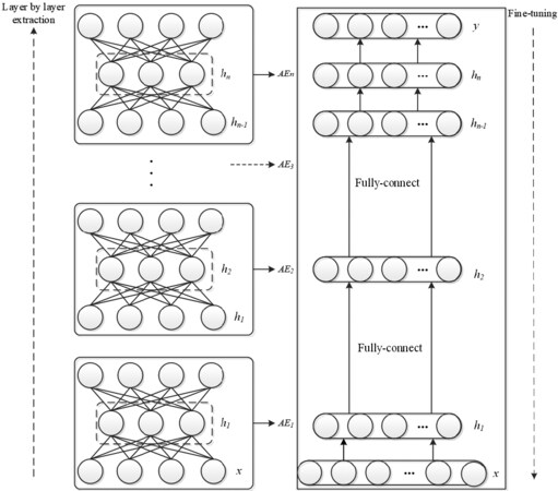
Figure 1. The structure diagram of deep neural network.

After layer-by-layer feature extraction, the Softmax classifier is added and applied. The network parameters can be fine-tuned with labeled data by using back propagation.

2.4 Federated learning

As shown in Figure 2, federated learning is essentially a distributed machine learning technology to train a unified network model by using data features provided by different organizers cooperatively. This paper uses the idea of federated learning to optimize federation of modular deep learning networks established under multiple working conditions and realizes federation between features through vertical federation.

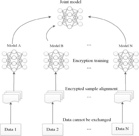
Figure 2. Vertical federated learning network.

3. MULTI-WORKING CONDITION FAULT DIAGNOSIS BASED ON MFLM

Due to variation of operating load, rolling bearings may operate in multiple working conditions. Figure 3 shows the normal probability plot of inner race fault data collected in a single working condition and multiple working conditions (Figure 3A and B, respectively). The x-axis of Figure 3 represents the data sorted in ascending order, while the y-axis represents the probability of a normal distribution. In the normal probability graph, if all sample points are near the solid line, the corresponding data obey normal distribution. Comparing Figure 3A and B, it can be seen that the data collected in multi-working condition violates the independent and identical distribution (i.i.d) assumption of machine learning algorithms, which is the basis of DNN for accurate feature extraction.

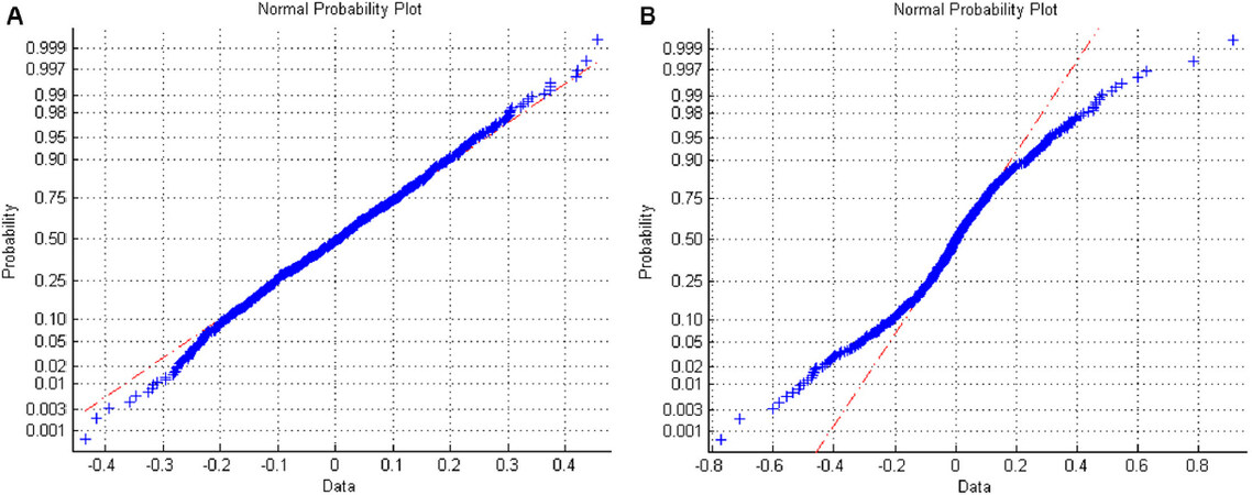
Figure 3. Comparison of normal probability graphs between single working condition data and multiple working condition data. (A) The normal probability graph of single working condition data. (B) The normal probability graph of multiple working condition data.

On the other hand, the existing modular neural network can only synthesize the sub-modules’ diagnosis results rather than integrate modules.

3.1 Constructed multi-working condition fault diagnosis network

To solve the above-mentioned problems, this section proposes a MFLM for multi-working condition fault diagnosis by designing a federation mechanism using dynamic routing technology. The overall framework of the MFLM-based method proposed in this paper is shown in Figure 4. The detailed steps of the proposed fault diagnosis for multiple working conditions are as follows:

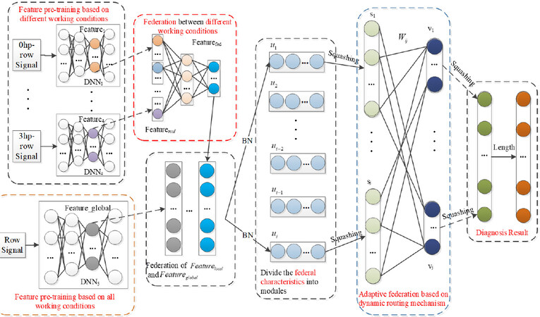
Figure 4. Network structure diagram for modular federated learning method.

Step 1. Data preprocessing

For the 1D vibration data collected by an accelerator sensor, the sliding time window technique is used for reshaping the original data in Equation (5), where l is the length of the time window, and the step length is step = 10.

(5) $$ \begin{equation} \begin{aligned} X_{\mathit {Train }}=\left[\begin{array}{cccc} x_{1} & x_{2} & \cdots & x_{l} \\ x_{\mathit{{step }} +1} & x_{\mathit {step }+2} & \cdots & x_{\mathit {step }+l} \\ \cdots & \cdots & \cdots & \cdots \\ x_{(\mathit{n} -1) \mathit{l} +1} & x_{(\mathit{n} -1) \mathit{l} +2} & \cdots & x_{\mathit{n l} } \end{array}\right] \\ \end{aligned} \end{equation} $$

n represents that the dataset X_Train contains n samples, each row in Equation (5) represents a sample, and the vector length of each sample is equal to the length of the sliding window.

Step 2. Construct a neural network for feature pre-extraction of each modular

Data collected from each working condition is fed into the input of a modular network. An additional modular network is established for combined data X_Train’ without data labels. The BN technique is adopted in DNN training. Taking the two hidden layers as an example, the layer-by-layer feature extraction using BN can be formulated as Equation (6)

(6) $$ \begin{equation} \begin{aligned} \mathit{Feature}_{i}=f\left(B N\left(W_{i, 2}\left(f\left(B N\left(W_{i, 1} x+b_{i, 1}\right)\right)\right)+b_{i, 2}\right)\right) \end{aligned} \end{equation} $$

Where x is the input sequence data, W_i,1 and W_i,2 represent the weight between the input and output of the ith DNN, b_i,1 and b_i,2 are the corresponding biases, and f(·) is the nonlinear activation function Relu.

The features extracted by multiple DNNs are spliced into Feature_mul. Feature_global is the global feature extracted by Equations (7) and (8). As shown in Equations (9) and (10), spliced feature Feature_mul is back propagated to each DNN for optimization, and the updated Feature_local can represent Feature_mul as much as possible.

(7) $$ \begin{equation} \begin{aligned} \mathit{Feature}_{\mathit{mul} }=\left[\mathit{Feature }_1 \mathit { Feature }_2, \mathit { Feature }_3, \mathit { Feature }_4\right] \end{aligned} \end{equation} $$

(8) $$ \begin{equation} \begin{aligned} \mathit { Feature }_{\mathit {global }}=\left[\mathit { Feature }_5\right] \end{aligned} \end{equation} $$

(9) $$ \begin{equation} \begin{aligned} h_1=f_{\theta, 1}\left(\mathit{Feature}_{\mathit{mul} }\right)=\sigma\left({ \mathit{W} }_1 { \mathit{Feature} }_{ {\mathit{mul} }}+b_1\right) \end{aligned} \end{equation} $$

(10) $$ \begin{equation} \begin{aligned} \mathit{Feature} _ {\mathit{global} }=f_{\theta, 2}\left(h_1\right) \end{aligned} \end{equation} $$

Where f_θ,1(·) represents the coding function of the first AE in SAE, f_θ,2(·) represents the coding function of the second AE, θ represents the coding parameter, and σ represents the non-linear activation function.

Step 3. Batch normalize data of different scales

Batch normalization is performed using Equations (11) and (12):

(11) $$ \begin{equation} \begin{aligned} \mathit{Feature} _s=\left[ { \mathit{Feature} }_{\mathit{loca} l }, \mathit{Feature}_{{\mathit{fed} }}\right] \end{aligned} \end{equation} $$

(12) $$ \begin{equation} \begin{aligned} \hat{\mathit{y} _l}=\mathit{γ} \frac{ \mathit{Feature} _s-E\left[\mathit{Feature}_s\right]}{\sqrt{\mathit { Var }\left[\mathit { Feature }_s\right]+\varepsilon }}+\beta \\ \end{aligned} \end{equation} $$

where E(·) and Var(·) are the mean and standard deviation of the input Feature_s. γ and β can be trained, and ε is a minimal number to ensure that the denominator is not 0.

Step 4. Federation of features at different scales

According to the local features of the single working condition extracted in Step 2 and the global feature of the multi-condition extracted by the global feature extraction network, a federation mechanism for the features at different scales is proposed. First, the local feature of the working condition label is federated to Feature^mul. Then, after the multi-layer feature optimization, the federated learning is performed with Feature^fed. The two features of different scales are merged to obtain Feature^s, and the normalized features after federation are divided into modules. Each module is a vector neuron, and the information involved is better than that of the traditional scalar neuron. The squashing function is added after each module to scale the length of the vector neuron obtained to within 0-1. The modules of the fusion feature are divided into adaptive federation through dynamic routing strategy to realize the adaptive allocation of the weights of the top-level modules.

The propagation of the capsules between two layers involves two stages: linear transformation and dynamic routing. Different from fully connected neural networks, each capsule is multiplied by an independent weight matrix to predict each high-level capsule, as shown in Equation (13).

(13) $$ \begin{equation} \begin{aligned} \hat{u}_{j|i}=\mathit{W} _{\mathit{i j} } u_\mathit{i} \end{aligned} \end{equation} $$

where u_i denotes the ith input capsule, W_ij is the weight matrix, and $$\hat{u}_{j|i}$$ denotes the prediction vectors.

Next, each prediction $$\hat{u}_{j|i}$$ propagates the features to all high-level capsules s_j by the dynamic routing technique, while the high-level capsule is the weighted sum over all its predictions, as shown in Equation (14).

(14) $$ \begin{equation} \begin{aligned} s_j = \displaystyle \sum_{i} \mathit{c} _{\mathit{i j} } \hat{u}_{j|i} \end{aligned} \end{equation} $$

where c_ij are coupling coefficients which satisfy the restriction of $$ \sum_\mathit{j} c_{\mathit{i j} }=1 $$. The coupling coefficients are determined by Equation (15):

(15) $$ \begin{equation} \begin{aligned} c_{\mathit{i j} } = \frac{\exp \left(b_{\mathit{i j} }\right)}{\displaystyle\sum_{j} \exp \left(b_{\mathit{i j} }\right)} \end{aligned} \end{equation} $$

where b_ij are the log prior probabilities that prediction $$\hat{u}_{j|i}$$ should be coupled to the high-level capsule s_j. Then, the squashing function shown in Equation (16) is used.

(16) $$ \begin{equation} \begin{aligned} \mathit{v} _\mathit{j} =\mathit{f} _s\left(s_j\right)=\frac{\left\|\mathit{s} _\mathit{j} \right\|^2}{1+\left\|s_\mathit{j}\right\|^2} \frac{s_\mathit{j}}{\left\|s_\mathit{j}\right\|} \end{aligned} \end{equation} $$

where s_j and v_j are the input and output of squashing, respectively. Parameter b_ij is updated, as shown in Equation (17).

(17) $$ \begin{equation} \begin{aligned} b_{\mathit{i j} } \gets b_\mathit{i j}+ \hat{u}_{j|i} \bullet \mathit{v} _\mathit{j} \end{aligned} \end{equation} $$

By iterating Equations (13)-(17) n times, the final feature v_j is obtained.

Step 5. Multi-working condition fault diagnosis

The new loss function defined in Equation (18) is designed for training of the network:

(18) $$ \begin{equation} \begin{aligned} M \arg \operatorname{inloss}\left(\mathit{v_j} \right)=R_c \mathit{max} \left(0, \mathit{m}^{+}-\left\|\mathit{v_j} \right\|\right)^2+\mathit{\mu} \left(1-R_c\right) \mathit{max} \left(0,\left\|v_j\right\|-\mathit{m} ^{-} \right)^2 \end{aligned} \end{equation} $$

where v_j represents the length of the federation module as well as the probability distribution of the fault diagnosis results, R_c is the target category of the current fault, and m⁺ = 0.9. m^- = 0.1 and μ = 0.6 are used to reduce the weight of loss without failure; the initial learning can be stopped by reducing the length of all units’ activation vectors.

3.2 Online fault diagnosis

Once online observation data X(t) are collected, they can be fed into the well trained MFLM model. The specific steps are as follows:

• Use the trained DNN₅ to perform global feature extraction on X(t), and fuse the trained Feature_local to obtain Feature_s.

• Send the fusion data Feature_s to the trained MFLM to realize fault diagnosis.

Figure 5 is the algorithm flow chart of the proposed method.

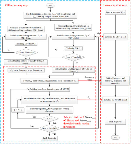
Figure 5. Algorithm block diagram for modular federated learning method.

4. EXPERIMENTAL RESULTS AND ANALYSIS

4.1 Bearing data description and experimental description

A benchmark dataset downloaded from Case Western Reserve University bearing center^[35] was used to test the effectiveness of the proposed method. The experimental platform is shown in Figure 6, including a 2 hp motor, power meter, electronic controller, torque sensor, and a load motor. The acceleration sensor was used to collect the motor drive end-bearing vibration signal under different load conditions in the experiment. The bearing’s health state was divided into four types: inner race fault (IF), outer race fault (OF), roller fault (RF), and normal condition (N). The size of each bearing fault in this dataset is 0.007, 0.014, 0.021, or 0.028 inches. The sampling frequency is 12 kHz. The bearing’s working conditions varies with the load as 0, 1, 2, or 3 hp.

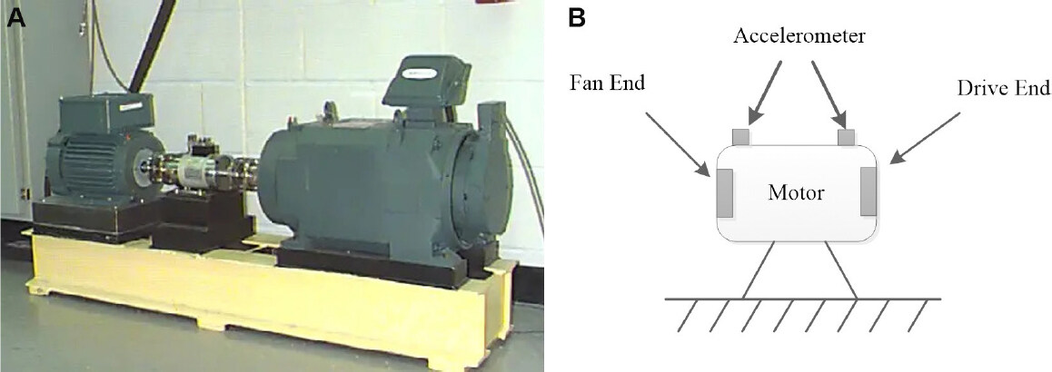
Figure 6. Bearing data collection equipment^[35]: (A) bearing data collection experiment platform diagram; and (B) location diagram of the acceleration sensor.

The multiple working conditions of the bearing are shown in Table 1.

Table 1

Working conditions of rolling bearings

Working condition	Load	Rotating speed (rpm)
Working condition 1	0	1797
Working condition 2	1	1772
Working condition 3	2	1750
Working condition 4	3	1730

Since the vibration data collected by the sensor are 1D sequence data, a sliding window with size 400 was used to preprocess the original sequence data. Each sliding window is a sample, and the sliding step length is 20.

To verify the effectiveness of the method in this paper, Experiments 1-9 were designed. The proposed method was compared with three existing fault diagnosis methods: the traditional DNN fault diagnosis method and the hierarchical DNN (HDNN) designed in^[14] and the fault diagnosis method proposed in^[24] (TICNN) were trained for a single working condition and used the trained network to test bearing faults under other working conditions. The network structure parameters are shown in Table 2.

Table 2

Network structure and parameters

Network model	Number of network layers	Learning rate	Activation function	Classifier	Optimization criteria
DNN	5	0.001	Relu	Softmax	Error back propagation algorithm
HDNN	6	0.001	Relu	Softmax	Error back propagation algorithm
TICNN	8	0.001	Relu	Softmax	Error back propagation algorithm
MFLM	6	0.001	Squash/Relu	Marginloss + Softmax	Dynamic routing strategy + error back propagation algorithm

DNN: Deep neural network; HDNN: hierarchical deep neural network; TICNN: convolution neural networks with training interference; MFLM: modular federated learning method.

To verify the influence of multi-condition data on the experimental results, Experiments 1-6 were designed, among which Experiments 1-3 are single-condition fault diagnosis experiments, while Experiments 4-6 are multi-condition fault diagnosis experiments. To verify the influence of the number of training samples on the fault diagnosis results, Experiments 7-9 were designed. The experimental design is shown in Table 3.

Table 3

Experimental design table

Experiment	Load state (hp)	Number of samples in each working condition module	Number of samples in the total module	Number of samples in the test set	Fault size (inch)	Fault type
Experiment 1	0	-	8000	1600	0.007	Normal, inner race, outer race, roller
Experiment 2	0	-	8000	1600	0.014	Normal, inner race, outer race, roller
Experiment 3	0	-	8000	1600	0.021	Normal, inner race, outer race, roller
Experiment 4	0/1/2/3	8000/8000/8000/8000	24000	1600	0.007	Normal, inner race, outer race, roller
Experiment 5	0/1/2/3	8000/8000/8000/8000	24000	1600	0.014	Normal, inner race, outer race, roller
Experiment 6	0/1/2/3	8000/8000/8000/8000	24000	1600	0.021	Normal, inner race, outer race, roller
Experiment 7	0/1/2/3	8000/8000/8000/8000	16000	1600	0.007	Normal, inner race, outer race, roller
Experiment 8	0/1/2/3	8000/8000/8000/8000	32000	1600	0.007	Normal, inner race, outer race, roller
Experiment 9	0/1/2/3	8000/8000/8000/8000	48000	1600	0.007	Normal, inner race, outer race, roller
Experiment 10	0/1/2/3	8000/8000/8000/8000	16000	1600	0.014	Normal, inner race, outer race, roller
Experiment 11	0/1/2/3	8000/8000/8000/8000	32000	1600	0.014	Normal, inner race, outer race, roller
Experiment 12	0/1/2/3	8000/8000/8000/8000	48000	1600	0.014	Normal, inner race, outer race, roller
Experiment 13	0/1/2/3	8000/8000/8000/8000	16000	1600	0.021	Normal, inner race, outer race, roller
Experiment 14	0/1/2/3	8000/8000/8000/8000	32000	1600	0.021	Normal, inner race, outer race, roller
Experiment 15	0/1/2/3	8000/8000/8000/8000	48000	1600	0.021	Normal, inner race, outer race, roller

4.2 Analysis of experimental results

4.2.1 Analysis of the experimental results of single working conditions and multiple working conditions

The experimental results of single working conditions and multiple working conditions are shown in Table 4. Experiments 1-3 are the experimental results of a single working condition. Experiment 1 is that the fault size is 0.007 inches, Experiment 2 is that the fault size is 0.014 inches, and Experiment 3 is that the fault size is 0.021 inches. Experiments 4-6 are the experimental results of multiple working conditions. Experiments 4-6 show that the fault size is 0.007, 0.014, and 0.021 inches, respectively.

Table 4

Comparison of experimental results between single working conditions and multiple working conditions

Experiment	DNN	HDNN	TICNN	MFLM
Experiment 1	90.57%	92.48%	94.86%	97.89%
Experiment 2	91.07%	92.86%	95.46%	98.23%
Experiment 3	92.36%	93.73%	96.28%	99.75%
Experiment 4	75.96%	85.17%	90.94%	93.13%
Experiment 5	83.39%	87.52%	91.36%	96.32%
Experiment 6	85.64%	89.72%	93.75%	97.56%

DNN: Deep neural network; HDNN: hierarchical deep neural network; TICNN: convolution neural networks with training interference; MFLM: modular federated learning method.

Comparing Rows 2 and 5 in Table 4, it can be seen that, when the size of the fault is the same, the multi-condition fault diagnosis accuracy of different networks is reduced compared to the single-condition fault accuracy. Similarly, comparing Rows 3 and 6, the same pattern can be found as in Rows 4 and 7. This shows that the data of multiple operating conditions caused the problem of feature extraction, which affected the diagnosis results. Therefore, it is of great practical significance to carry out fault diagnosis research under multiple working conditions. Comparing the Columns 2 and 5 of Row 4, it can be seen that the MFLM method proposed in this paper has fault diagnosis accuracy 7.39% higher than that of the traditional DNN method when the fault size is 0.021 inches. In the fault diagnosis of industrial field, it is more difficult to improve the accuracy to more than 95%. MFLM not only improves the accuracy to more than 95%, but also reaches 99.75%, so it is more likely to be valued by engineers.

To improve the readability of the experiment results listed in Table 4, Figure 7 shows the fault diagnosis classification chart taking Experiment 6 as an example. The classification results are represented by blue stars in the figure. The red circles represent the true fault categories of the sample. The coincidence of red circle and blue star indicates that the classification is correct. Figure 7A-D corresponds to Row 7 in Table 4. Figure 7A is the result of traditional DNN fault diagnosis. Figure 7B is the result of HDNN fault diagnosis. Figure 7C is the result of TICNN fault diagnosis. Figure 7D is the result of MFLM fault diagnosis.

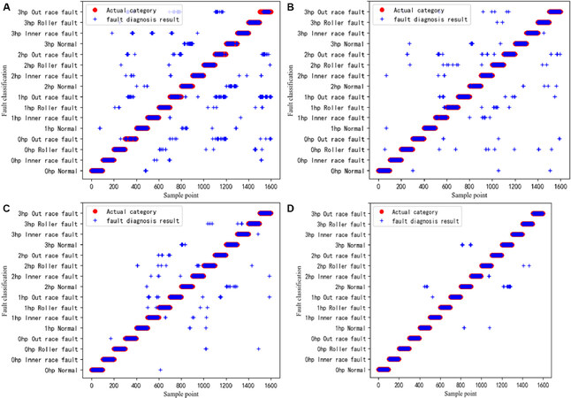
Figure 7. Fault diagnosis classification diagram. The fault diagnosis result of multiple working conditions with a fault size of 0.021 inches. (A) Shows the fault diagnosis classification diagram of deep neural network; (B) shows the fault diagnosis classification diagram of hierarchical deep neural network; (C) shows the fault diagnosis classification diagram of convolution neural networks with training interference; and (D) shows the fault diagnosis classification diagram of modular federated learning method.

Figure 7A shows that the blue stars are dense, which indicates that the misclassification rate is relatively high. Figure 7B has fewer blue stars than Figure 7A, indicating that HDNN’s classification effect is better than the traditional DNN. This is because HDNN adopts a hierarchical fault diagnosis method, which first diagnoses the working condition category, and then diagnoses the fault category. Figure 7D shows that MFLM has the fewest blue stars, which means that the misclassification rate is the lowest. This explains the superiority of the modular neural network in fault diagnosis of multiple working conditions.

4.2.2 Analysis of fault diagnosis results of multiple working conditions with different sample sizes

The number of training samples is an important factor affecting the effectiveness of fault diagnosis. It is difficult to obtain high-quality labeled fault samples in industrial sites. Therefore, to verify the results of different sample sizes for multi-condition fault diagnosis, the number of samples for each type of fault in Experiment 7-9 is 1000, 2000, and 3000, respectively, while the size of the fault is 0.007, 0.014, and 0.021 inches, respectively. The experimental results are shown in Table 5.

Table 5

Multi-working condition fault diagnosis results with different numbers of training samples

Experiment	DNN	HDNN	TICNN	MFLM
Experiment 7	75.93%	83.14%	89.06%	91.97%
Experiment 8	77.02%	86.01%	91.77%	93.81%
Experiment 9	79.68%	88.64%	93.01%	95.03%
Experiment 10	82.87%	87.05%	91.34%	94.39%
Experiment 11	85.43%	88.92%	93.27%	97.15%
Experiment 12	86.52%	91.17%	95.09%	97.91%
Experiment 13	85.32%	89.19%	94.32%	97.11%
Experiment 14	87.53%	91.14%	95.96%	98.29%
Experiment 15	89.03%	94.29%	97.83%	99.07%

DNN: Deep neural network; HDNN: hierarchical deep neural network; TICNN: convolution neural networks with training interference; MFLM: modular federated learning method.

Comparing Columns 2 and of Row 4 of Table 5, it can be seen that, when the fault size is 0.007 inches and the number of samples without working condition labels is 48,000, the multi-working condition diagnosis accuracy of MFLM can reach 95.03%. The diagnostic accuracy of the traditional DNN method is lower than 80%. Comparing Columns 4 and 5 of Row 4, it can be seen that, although the existing TICNN method can achieve more than 90% accuracy in multi-condition diagnosis, it is still lower than the MFLM method. This illustrates the effectiveness of modular federation in MFLM. Comparing Rows 4 and 10, it can be seen that, when the fault size is 0.021 inches and the number of samples without working conditions is 16,000 and 48,000, the greater is the number of samples, the higher is the accuracy of fault diagnosis. In fault diagnosis, the number of samples is an important factor that affects the result of fault diagnosis. Comparing Columns 4 and 5 of Row 8, it can be seen that, when the fault size is 0.021 inches and the number of samples without working conditions is 16,000, the diagnostic accuracy of MFLM is 97.11%, which is 2.79% higher than that of TICNN. The accuracy is increased to more than 95%, which is a very important improvement in engineering. Row 10 of Table 5 shows that, when the fault size is 0.021 inches and the number of samples without working conditions is 48,000, while the diagnostic accuracy of the various fault diagnosis methods was improved, the diagnostic accuracy of MFLM could reach 99.07%, which illustrates the superiority of the method proposed in this paper.

To improve the readability of the experiment results listed in Table 5, Figure 8 shows the fault diagnosis classification chart taking Experiment 15 as an example. Figure 8A-D correspond to Row 10 in Table 5. Figure 8A is the result of traditional DNN fault diagnosis. Figure 8B is the result of HDNN fault diagnosis. Figure 8C is the result of TICNN fault diagnosis. Figure 8D is the result of MFLM fault diagnosis.

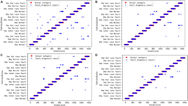
Figure 8. Fault diagnosis classification diagram. The fault size is 0.021 inches, the number of samples without working conditions is 48,000, and the fault diagnosis results are shown under multiple working conditions. (A) Shows the fault diagnosis classification diagram of deep neural network; (B) shows the fault diagnosis classification diagram of hierarchical deep neural network; (C) shows the fault diagnosis classification diagram of convolution neural networks with training interference; and (D) shows the fault diagnosis classification diagram of modular federated learning method.

Figure 8A shows that the blue stars are dense, which indicates that the misclassification rate is relatively high. Figure 8B has fewer blue stars than Figure 8A, indicating that HDNN’s classification effect is better than that of the traditional DNN. This is because HDNN adopts a hierarchical fault diagnosis method, which first diagnoses the working condition category, and then diagnoses the fault category. Figure 8D shows that MFLM has the fewest blue stars, which means that the misclassification rate is the lowest. This explains the superiority of modular neural network in fault diagnosis of multiple working conditions. Figure 9 shows a comparative bar graph of all experimental results.

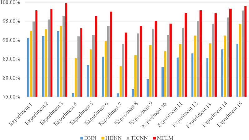
Figure 9. Comparison of different fault diagnosis method for rolling bearing.

5. CONCLUSIONS

Aiming at improving the low generalization ability of traditional neural networks when solving multi-working condition problems, this paper designs a modular federated neural network based on dynamic routing technology to design a federated mechanism of multiple modular networks. Using the proposed method, bearing fault diagnosis under multiple working conditions can be well diagnosed without requiring an additional module recognition stage.

REFERENCES

1. Djelloul I, Sari Z, Sidibe IDB. Fault diagnosis based on the quality effect of learning algorithm for manufacturing systems. Proceedings of the Institution of Mechanical Engineers, Part I: Journal of Systems and Control Engineering 2019;233:801-14.
2. Li J, Yao X, Wang X, Yu Q, Zhang Y. Multiscale local features learning based on BP neural network for rolling bearing intelligent fault diagnosis. Measurement 2020;153:107419.
3. Xu X, Zhao Z, Xu X, et al. Machine learning-based wear fault diagnosis for marine diesel engine by fusing multiple data-driven models. Knowledge-Based Systems 2020;190:105324.
4. Hoang D, Kang H. A survey on Deep Learning based bearing fault diagnosis. Neurocomputing 2019;335:327-35.
5. Xu Z, Li C, Yang Y. Fault diagnosis of rolling bearing of wind turbines based on the Variational Mode Decomposition and Deep Convolutional Neural Networks. Applied Soft Computing 2020;95:106515.
6. Zhou F, Zhang Z, Chen D. Real-time fault diagnosis using deep fusion of features extracted by parallel long short-term memory with peephole and convolutional neural network. Proceedings of the Institution of Mechanical Engineers, Part I: Journal of Systems and Control Engineering 2021;235:1873-97.
7. Li C, Bao Z, Li L, Zhao Z. Exploring temporal representations by leveraging attention-based bidirectional LSTM-RNNs for multi-modal emotion recognition. Information Processing & Management 2020;57:102185.
8. Kong X, Mao G, Wang Q, Ma H, Yang W. A multi-ensemble method based on deep auto-encoders for fault diagnosis of rolling bearings. Measurement 2020;151:107132.
9. Liu H, Qu X, Gao L, et al. Characterization of a Bacillus subtilis surfactin synthetase knockout and antimicrobial activity analysis. J Biotechnol 2016;237:1-12.
10. Shao H, Jiang H, Wang F, Zhao H. An enhancement deep feature fusion method for rotating machinery fault diagnosis. Knowledge-Based Systems 2017;119:200-20.
11. Sun W, Chen J, Li J. Decision tree and PCA-based fault diagnosis of rotating machinery. Mech Syst Signal Process 2007;21:1300-17.
12. Song B, Tan S, Shi H. Key principal components with recursive local outlier factor for multimode chemical process monitoring. Journal of Process Control 2016;47:136-49.
13. Liu H, Li L, Ma J. Rolling bearing fault diagnosis based on STFT-deep learning and sound signals. Shock and Vibration 2016;2016:1-12.
14. Zhou F, Gao Y, Wen C. A novel multimode fault classification method based on deep learning. Journal of Control Science and Engineering 2017;2017:1-14.
15. Chen X, Zhang B, Gao D. Bearing fault diagnosis base on multi-scale CNN and LSTM model. J Intell Manuf 2021;32:971-87.
16. Gu X, Zhou B. Multimodal industrial process fault detection based on LNS-DEWKECA. Control and Decision 2020;35:1879-86.
17. Che C, Wang H, Ni X, Fu Q. Domain adaptive deep belief network for rolling bearing fault diagnosis. Computers & Industrial Engineering 2020;143:106427.
18. Qiao H, Wang T, Wang P, Zhang L, Xu M. An adaptive weighted multiscale convolutional neural network for rotating machinery fault diagnosis under variable operating conditions. IEEE Access 2019;7:118954-64.
19. Zhao B, Zhang X, Zhan Z, Pang S. Deep multi-scale convolutional transfer learning network: a novel method for intelligent fault diagnosis of rolling bearings under variable working conditions and domains. Neurocomputing 2020;407:24-38.
20. Han S, Yu Y, Tang T, et al. Measurement of weld pool oscillation for pulsed GTAW based on laser vision. Microcomputer Applications 2019;35:8-13.
21. Jacobs RA, Jordan MI, Nowlan SJ, Hinton GE. Adaptive mixtures of local experts. Neural Comput 1991;3:79-87.
22. Andreas J, Rohrbach M, Darrell T, Klein D. Neural module networks. Proceedings of the IEEE Conference on Computer Vision and Pattern Recognition 2016:39-48.
23. Zhang W, Li C, Peng G, Chen Y, Zhang Z. A deep convolutional neural network with new training methods for bearing fault diagnosis under noisy environment and different working load. Mech Syst Signal Process 2018;100:439-53.
24. Zhao X, Xiao D. Fault diagnosis of nonlinear systems based on modular fuzzy neural networks. Control Theory and Applications 2001;18:395-400.
25. Bo YC, Qiao JF, Yang G. A Modular Neural Networks ensembling method based on fuzzy decision-making. 2011 International Conference on Electric Information and Control Engineering Wuhan, China. IEEE; 2011. pp. 1030-4.
26. Yan Z, Zhang H, Piramuthu R, et al. HD-CNN: hierarchical deep convolutional neural networks for large scale visual recognition. Proceedings of the IEEE International Conference on Computer Vision (ICCV) 2015. pp. 2740-8.
27. Geng Z, Ding N, Han Y. Fault diagnosis of converter based on wavelet decomposition and BP neural network. 2019 Chinese Automation Congress (CAC) Hangzhou, China. IEEE; 2020. pp. 1273-6.
28. Sabour S, Frosst N, Hinton GE. Dynamic routing between capsules. arXiv preprint arXiv:1710.09829 2017.
29. Chen T, Wang Z, Yang X, Jiang K. A deep capsule neural network with stochastic delta rule for bearing fault diagnosis on raw vibration signals. Measurement 2019;148:106857.
30. Li L, Zhang M, Wang K. A fault diagnostic scheme based on capsule network for rolling bearing under different rotational speeds. Sensors (Basel) 2020;20:1841.
31. Zhu Z, Peng G, Chen Y, Gao H. A convolutional neural network based on a capsule network with strong generalization for bearing fault diagnosis. Neurocomputing 2019;323:62-75.
32. Rumelhart DE, Hinton GE, Williams RJ. Learning representations by back-propagating errors. Nature 1986;323:533-6.
33. Ioffe S, Szegedy C. Batch normalization: accelerating deep network training by reducing internal covariate shift. Proceedings of the 32nd International Conference on Machine Learning 2015. pp. 448-56.
34. Wang J, Li S, An Z, Jiang X, Qian W, Ji S. Batch-normalized deep neural networks for achieving fast intelligent fault diagnosis of machines. Neurocomputing 2019;329:53-65.
35. Bearingdata Centre. Case Western Reserve University. Available: http://csegroups.case.edu/bearingdatacenter/home. [Last accessed on 15 Oct 2021].
Cite This Article
Export citation file: BibTeX | RIS
OAE Style
Zhou F, Zhang Z, Li S. Research on federated learning method for fault diagnosis in multiple working conditions. Complex Eng Syst 2021;1:7. http://dx.doi.org/10.20517/ces.2021.08
AMA Style
Zhou F, Zhang Z, Li S. Research on federated learning method for fault diagnosis in multiple working conditions. Complex Engineering Systems. 2021; 1(2): 7. http://dx.doi.org/10.20517/ces.2021.08
Chicago/Turabian Style
Zhou, Funa, Zhiqiang Zhang, Sijie Li. 2021. "Research on federated learning method for fault diagnosis in multiple working conditions" Complex Engineering Systems. 1, no.2: 7. http://dx.doi.org/10.20517/ces.2021.08
ACS Style
Zhou, F.; Zhang Z.; Li S. Research on federated learning method for fault diagnosis in multiple working conditions. Complex. Eng. Syst. 2021, 1, 7. http://dx.doi.org/10.20517/ces.2021.08
About This Article
Copyright
Data & Comments
Data
Cite This Article 23 clicks
Like This Article 37
likes
Comments
Comments must be written in English. Spam, offensive content, impersonation, and private information will not be permitted. If any comment is reported and identified as inappropriate content by OAE staff, the comment will be removed without notice. If you have any queries or need any help, please contact us at support@oaepublish.com.