Fuzzy reduced-order filtering for nonlinear parabolic PDE systems with limited communication

1. INTRODUCTION

Numerous processes in industry are related not only to time but also to spatial location^[1–3], such as nuclear reaction processes, fluid heat exchange processes and biological systems^[4–6]. These systems are called distributed parameter systems, usually described by partial differential equations (PDE)^[7–9]. According to the different characteristics of the spatial differential operators, the PDE systems can be further divided into three categories, namely, hyperbolic^[7], parabolic^[8] and elliptic^[9]. In particular, parabolic PDEs can be applied to express the dynamic of industrial processes involve diffusion-convection-reaction processes, such as crystal growth processes, semiconductor thermal processes and wavy behavior in chemistry^[10,11]. Therefore, control/filtering studies for parabolic PDE systems have attracted extensive attention^[12–17]. For example, Wang et al.^[12] introducted the estimator-based H_∞ sampled-data fuzzy control for nonlinear parabolic PDE systems; Zhang et al.^[16] addressed the controller design under mobile collocated actuators and sensors; Song et al.^[17] discussed the reliable H_∞ filter design for PDE system with Markovian jumping sensor faults, which stimulated the author’s interest in PDE systems.

In another research field, numerous feasible methods have been developed to solve the analysis and synthesis problem of nonlinear systems. Among them, Takagi-Sugeno (T-S)fuzzy model is widely adopted as an effective method for stability analysis of nonlinear systems^[18], which can express any smooth nonlinear function with arbitrary accuracy in any convex compact region^[19,20]. In addition, the stability analysis problem of fuzzy control/filtering can be solved by employing the linear matrix inequality (LMI) methods^[21]. Based on these advantages of the fuzzy model, many studies have been conducted to apply fuzzy models in controller/filter design for parabolic PDE systems^[22,23]. Kerschbaum et al.^[22] addressed the backstepping control for parabolic PDE systems; Qiu et al.^[23] addressed the distributed adaptive output feedback consensus problem for parabolic PDE systems.

Meanwhile, the above study mainly used the traditional time-triggered (periodical sampling) network transmission method. The periodic sampling will lead to waste of the network resources and redundancy of transmission signals^[24]. Therefore, to better save communication resources, Tabuada^[25] proposed an event-triggered mechanism (ETM) that can effectively save network transmission resources, which can determine whether to transmit data according to different trigger conditions^[26–32]. For example, Wang et al.^[26] developed an output-feedback backstepping control method for PDE systems with ETM; based on ETM, Ji et al.^[27] considered the filtering control for PDE systems. These results prove that, compared to the traditional periodic sampling, ETM can effectively reduce the burden of network bandwidth and improve resource utilization.

Many nonlinear systems are multi-input and multi-output systems^[33–37], which the system models are often complex and diverse, how to design simple controllers/filters to meet the corresponding needs. Recently, Su et al.^[38] proposed a reduced-order filter (ROF) design method, namely, the order of the ROF is lower than the original plant, which will be more favorable for the real-time filtering procedure because some redundancy and extra calculation can be effectively avoided by this flter^[39,40]. However, as far as the author knows, there is little work on the design of fuzzy ROF for PDE systems, which arouses the author’s interest.

Based on the above discussion, this article intends to design a fuzzy ROF with H_∞ performance for the PDE systems, which its main contributions are as follows:

(1) Different from the fuzzy ROF design^[38], the influence of space position is fully considered in the system model and filter design process, the considerations are more comprehensive. Meanwhile, the ROF is designed on the basis of the early work^[17], which makes the complex engineering mathematical model more simplified and flexible.

(2) Compared with time-triggered fuzzy filter design^[41], the ETM is applied to determine whether to send a sampled signal, which can effectively solve the problem of signal resource transmission in the network.

Organization: Section 2 provides a problem statement and gives relevant definitions and lemmas, which include fuzzy system models, ROF structures and ETM. Section 3 is the main result of this paper, which include stability analysis and ROF design. A numerical example to prove the practicability of the obtained results in Section 4. Section 5 gives conclusions and future research directions.

Notations:$$ \mathbb{R}^{n} $$ represents n-dimensional Euclidean space; $$ \mathbb{H}^{n} $$ indicates Hilbert space; The notation N^T and N^–1 stand for the transpose and inverse matrix of the matrix N, respectively; X > 0 (≥ 0) means the matrix X is positive-definite (semi-definite); for ease of expression, define ψ = ψ(x,t) φ = φ(x,t), ω = ω(x,t), $$ \varphi_{o}=\varphi_{o}(x,t),\varphi_{m}=\varphi_{m}(x,t),\psi_{t}=\frac{\partial \psi (x,t)}{\partial t},\psi_{xx}=\frac{\partial \psi (x,t)}{\partial x^{2}} $$, $$ \theta =\theta (x,t),h_{i}=h_{i}(\theta (x,t)),\hat{\psi}=\hat{\psi}(x,t),\hat{\varphi}_{m}=\hat{\psi}_{m}(x,t) $$, $$ \hat{\varphi}_{o}=\hat{\psi}_{o}(x,t),\hat{\psi}_{t}=\frac{\partial \hat{\psi}(x,t)}{\partial t},\hat{\psi}_{xx}=\frac{\partial \hat{\psi}(x,t)}{\partial x^{2}},\varphi_{m}(t_{knT})=\varphi_{m}(x,t_{k}T+nT) $$, $$ \varphi_{m}(t_{kT})=\varphi_{m}(x,t_{k}T),e(i_{kT})=e_{k}(x,i_{k}T), \varphi_{mh}=\varphi_{m}(x,t-h(t)),e_{h}=e_{k}(x,t-h(t)) $$, $$ \eta_{h}=\eta(x,t-h(t)),\eta_{th}=\eta(x,t-h),\eta_{\theta}=\eta(x,\theta),\eta(s)=\eta(x,s) $$, $$ \eta_{s}(s)=\frac{\partial \eta (x,s)}{\partial s},\xi =\xi (x,t) $$; Matrices not explicitly stated in the text are assumed to have the appropriate dimensionality.

2. PROBLEM STATEMENT

3. RESULTS

In this section, the asymptotically stable condition of the error system (13) is obtained in Theorem 1. The ROF parameters will be obtained by the LMI method in Theorem 2.

Theorem 1. For given scalars γ > 0, ε > 0 and h > 0, error system (13) is asymptotically stable with H∞ performance, if there exist matrices Ω > 0, S satisfying $$ S\bar{\Theta }\ge 0 $$, P > 0, Q > 0, T₁> 0 and G satisfy the following inequality for all i ∈ {1,2, ·…, r}, j ∈ {1,2, …, r}:

where

Proof. The Lyapunov function is selected as follows

where

The derivative of V(t) is as follows:

According to Lemmas 1 and 2, the following inequality can be obtained

Furthermore, from (13), we can get:

Under the boundary conditions (2), by partial integration we can obtain:

Consider the ETM (10), define:

and

Combining (18)-(21) and schur complement, we have:

When ω(x, t) ≡ 0 and according to Theorem 1 and Definition 1, with the processing method ^[17], we can get the error system (13) is asymptotically stable. Under zero initial condition, one can obtain:

which indicates that

which completes the proof.☐

Next, solving several LMIs to obtain the parameters of the designed ROF, the main results are as follows:

Theorem 2. For given scalars ε ∈ [0,1), γ > 0, h > 0, if there exist real matrices W > 0, Q > 0, R > 0, Ω > 0, $$ S_{1}> 0, T_{1}> 0, \tilde{A}_{kj},\tilde{B}_{kj},\tilde{C}_{kj} $$ satisfy the following matrix inequations for i ∈ {1, 2, …, r}, j ∈ {1, 2, …, r} :

where

then the designed ROF (6) can be obtained by the following relation:

Proof. If the conditions (14)-(16) in Theorem 1 are satisfied, then the non-singular matrix can be divided into:

where

For the purpose of proving that S₂ is non-singular, define:

and

Since S > 0, it is easily to obtain M > 0 for σ > 0. Consequently, it is convenient to verify that M₂ is non-singular for arbitrarily σ > 0 and the above expression is feasible with S. In general, it is assumed that S₂ is non-singular subject to M₂. Based on the above discussion the following definitions can be obtained:

and

Then, we can get:

Pre- and post-multiply both sides of (16) with diag {U^T U^T I_1×6} and its transpose, respectively. If (32)-(34) is considered, then the inequality (26)-(28) can hold. Therefore, the error system (13) can be guaranteed to be asymptotically stable with H∞ performance. In addition, (33) is equivalent to

Thus, the A_kj, B_kj, C_kj in (6) can be obtained by (35). In case of general, let $$ S_{2}^{-T}S_{3}=I $$, we obtain (29), which can be adopted to construct the ROF in (6). This completes the proof.☐

Remark 3. It is noted that the matrix $$ \mathcal{H} $$ presented in Theorem 2 plays a pivotal role in the filter design problem because it is used as a reduced-order factor. When $$ \mathcal{H} $$ is a unit matrix, the designed filter is a full-order filter (FOF). The presence of $$ \mathcal{H} $$ allows for efficient conversion between ROF and FOF.

4. SIMULATION EXAMPLE

In this section, to illustrate the effectiveness of the proposed method, the ROF design problem is studied for the FHN equation, which is a widely adopted model of excitable medium fluctuations in chemistry and can be described as follows:

with boundary (2) and initial conditions

The following output and measurement signals are given:

where $$ \psi=col[\psi_{1}\quad \psi_{2}] $$, $$ \omega =col [\omega_{1}\quad \omega_{2}] $$, $$ \omega_{1}=0.01\sin(x)e^{-t} $$, $$ \omega_{2}=0.1\sin(x)e^{-t} $$, $$ D=-0.05I $$, $$ C2=-0.01I $$, E = I.

The systems (36) can be represented by the following fuzzy rule ^[43]:

Plant Rule 1: IF ξ(ψ₁) is “Big”, THEN

Plant Rule 2: IF ξ(ψ₁) is “Small”, THEN

where $$ \xi(\psi_{1})=\psi_{1}^{2} $$, $$ A_{1}=\begin{bmatrix} -\chi -1.2 & -1\\ 0 & -0.1\end{bmatrix} $$, $$ A_{2}=\begin{bmatrix} -1.2 & -1\\ 0 & -0.1\end{bmatrix} $$ and $$ C_{1}=\begin{bmatrix} 1.2 & 0\\ 0.8 & 0\end{bmatrix} $$ with $$ \chi \triangleq \mathrm{max}_{\psi 1}\psi _{1}^{2} $$, ψ₁ ∈ [–1.5,1.5], we can get χ= 2.55 . The fuzzy membership function can be obtained:

Thus, the following T-S fuzzy model is written as follows:

where $$ A_{1}=\begin{bmatrix} -3.45 & -1\\ 0 & -0.1\end{bmatrix} $$, $$ A_{2}=\begin{bmatrix} -1.2 & -1\\ 0 & -0.1\end{bmatrix} $$. Assume h = 1ms, ε = 0.05, Θ = 1, Θ_k= 0.5 and by solving several LMI in Theorem 2, the parameters of the ROF are shown as follows:

Finally, to observe the H∞ performance more conveniently, define

Simulation result: the trajectory of the error system (13) is shown in Figures 1 and 2. Figure 3 shows the release moment under the ETM, the trajectory of ξ (t) defined in (37) is shown in Figure 4. It can be observed that the filtering error system is asymptotically stable with H∞ performance. Moreover, the designed ETM (7) can effectively reduce the amount of network signal transmissions and improve the efficiency of network resources utilization.

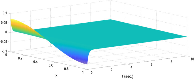
Figure 1. The trajectory of z̃_o1 (x, t).

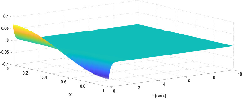
Figure 2. The trajectory of z̃_o2 (x, t).

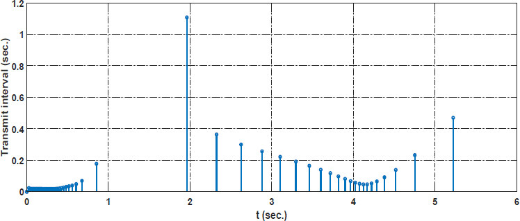
Figure 3. Release instants and release interval.

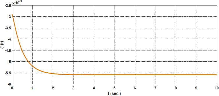
Figure 4. The trajectory of ξ (t) under zero initial condition.

Remark 4. Inspired by ETM ^[25], we introduce an ETM in the signal transmission process. Compared with the original TTCM^[41], it can effectively reduce the number of signal transmission and improve the network resource utilization. On the other hand, Song et al.^[17] considered filtering for parabolic PDE systems, but did not consider the problem of ROF design. Compared with Example 2^[17], the method proposed in this paper can achieve the same filtering function and the order of the filter is lower than the order of the plant, which simplifies the filter design.

5. CONCLUSIONS

This paper investigates the design method of fuzzy ROF based on ETM for nonlinear parabolic PDE systems. First, a T-S fuzzy model has been considered to reconstruct the nonlinear parabolic PDE systems. In addition, an ETM has been employed to reduce the amount of network transmission data to improve the network resource utilization. Then, the parameters of the designed ROF have been obtained by solving several LMIs based on Lyapunov direct method. Finally, the effectiveness of the proposed method is illustrated by simulation experiments. However, due to the time-delay phenomenon, the systems output signal is difficulty to keep synchronized through the network transmission between the filter and the plant. Therefore, in future studies, we will further consider asynchronous ROF for fuzzy PDE systems, which will be a more interesting topic.

REFERENCES

1. Ray W. Advanced process control. New York: McGraw Hill; 1981.
2. Sun J, Wang X, Xiong N, Jie S. Learning sparse representation with variational auto-encoder for anomaly detection. IEEE Access 2018;6:33353-61.
3. Fang W, Yao X, Zhao X, Yin J, Xiong N. A stochastic control approach to maximize profit on service provisioning for mobile cloudlet platforms. IEEE Trans Syst Man Cybern 2016;48:522-34.
4. Ferragut A, Paganini F. Fluid models of population and download progress in P2P networks. IEEE Trans Control Netw Syst 2016;3:34-45.
5. Lu X, Zou W, Huang M. A novel spatiotemporal LS-SVM method for complex distributed parameter systems with applications to curing thermal process. IEEE Trans Industr Inform 2016;12:1156-65.
6. Song X, Wang M, Ahn CK, Song S. Finite-time fuzzy bounded control for semilinear PDE systems with quantized measurements and Markov jump actuator failures. IEEE Trans Cybern 2021; doi: 10.1109/TCYB.2021.3049842.
7. Karafyllis I, Bekiaris LN, Papageorgiou M. Feedback control of nonlinear hyperbolic PDE systems inspired by traffic flow models. IEEE Trans Automat Contr 2019;64:3647-62.
8. Wu H, Wang J, Li H. Fuzzy boundary control design for a class of nonlinear parabolic distributed parameter systems. IEEE Trans Fuzzy Syst 2014;22:642-52.
9. Froese BD, Oberman AM, Salvador T. Numerical methods for the 2-Hessian elliptic partial differential equation. IMA Journal of Numerical Analysis 2017;37:209-36.
10. Christofides P. Nonlinear and robust control of PDE systems: methods and applications to transport-reaction processes. USA: Springer Science & Business Media; 2001.
11. Deng H, Li H, Chen G. Spectral-approximation-based intelligent modeling for distributed thermal processes. IEEE Trans Control Syst Technol 2005;13:686-700.
12. Wang Z, Wu H, Li H. Estimator-based H∞ sampled-data fuzzy control for nonlinear parabolic PDE systems. IEEE Trans Syst Man Cybern 2020;50:2491-500.
13. Wang Z, Wu H. Sampled-data fuzzy control with guaranteed cost for nonlinear parabolic PDE systems via static output feedback. IEEE Trans Fuzzy Syst 2020;28:2452-65.
14. Deutscher J. Robust cooperative output regulation for a network of parabolic PDE systems. IEEE Trans Automat Contr 2021; doi: 10.1109/TAC.2021.3079352.
15. Wang J. Dynamic boundary fuzzy control design of semilinear parabolic PDE systems with spatially noncollocated discrete observation. IEEE Trans Cybern 2019;49:3041-51.
16. Zhang X, Wu H. Fuzzy control design of nonlinear time-delay parabolic PDE systems under mobile collocated actuators and sensors. IEEE Trans Cybern 2020; doi: 10.1109/TCYB.2020.3020087.
17. Song X, Wang M, Zhang B, Song S. Event-triggered reliable H∞ fuzzy filtering for nonlinear parabolic PDE systems with Markovian jumping sensor faults. Information Sciences 2020;510:50-69.
18. Takagi T, Sugeno M. Fuzzy identification of systems and its applications to modeling and control. IEEE Trans Syst Man Cybern 1985;15:116-32.
19. Tsai SH. Robust H∞ stabilization conditions for a class of uncertain T-S fuzzy neutral systems with disturbance. Neurocomputing 2016;193:68-80.
20. Chen Z, Zhang B, Zhang Y, Ma Q, Zhang Z. Event-based control for networked T-S fuzzy systems via auxiliary random series approach. IEEE Trans Cybern 2018;50:2166-75.
21. Sheng Y, Lewis FL, Zeng Z, Huang T. Stability and stabilization of Takagi-Sugeno fuzzy systems with hybrid time-varying delays. IEEE Trans Fuzzy Syst 2019;27:2067-78.
22. Kerschbaum S, Deutscher J. Backstepping control of coupled linear parabolic PDEs with space and time dependent coefficients. IEEE Trans Automat Contr 2020;65:3060-7.
23. Qiu Q, Su H, Zeng Z. Distributed adaptive output feedback consensus of parabolic PDE agents on undirected networks. IEEE Trans Cybern 2021; doi: 10.1109/TCYB.2021.3050729.
24. Bing L, Zhu F, Zhang J, et al. A time-driven data placement strategy for a scientific workflow combining edge computing and cloud computing. IEEE Trans Industr Inform 2019;15:4254-65.
25. Tabuada P. Event-triggered real-time scheduling of stabilizing control tasks. IEEE Trans Automat Contr 2007;52:1680-5.
26. Wang J, Krstic M. Event-triggered output-feedback backstepping control of sandwiched hyperbolic PDE Systems. IEEE Trans Automat Contr 2021; doi: 10.1109/TAC.2021.3050447.
27. Ji H, Zhang H, Cui B. Event-triggered H∞ filtering control for a class of distributed parameter systems with Markovian switching topology. J Franklin Inst 2018;355:5928-56.
28. Ji H, Cui B. Event-generator-based H∞ control of fuzzy distributed parameter systems. Fuzzy Sets Syst 2021; doi: 10.1016/j.fss.2021.03.012.
29. Mu W, Qiu F, Zhuang B, Chen L. Optimal actuator switching synthesis of observer-based event-triggered state feedback control for distributed parameter systems. J Franklin Inst 2021;358:384-99.
30. Liang H, Liu G, Zhang H, Huang T. Neural-network-based event-triggered adaptive control of nonaffine nonlinear multiagent systems with dynamic uncertainties. IEEE Trans Neural Netw Learn Syst 2021;32:2239-50.
31. Liang H, Guo X, Pan Y, Huang T. Event-triggered fuzzy bipartite tracking control for network systems based on distributed reduced-order observers. IEEE Trans Fuzzy Syst 2021;29:1601-14.
32. Ji H, Cui B, Liu X. Event-triggered predictor-based control of distributed parameter systems. IET Control Theory & Applications 2021;15:721-36.
33. Liu L, Gao T, Liu Y, et al. Time-varying IBLFs-based adaptive control of uncertain nonlinear systems with full state constraints. Automatica 2021;129:109595.
34. Liu L, Liu Y, Chen A, et al. Integral barrier Lyapunov function-based adaptive control for switched nonlinear systems. Sci China Life Sci 2020;63:1-14.
35. Liang H, Zhou Y, Zhang H. Containment control for singular multi-agent systems with an internal model compensator. Sci China Life Sci 2020;63:1-3.
36. Li H, Liu J, Liu W, et al. A dimensionality reduction-based multi-step clustering method for robust vessel trajectory analysis. Sensors 2017;17:1792.
37. Zhang B, Xu S, Ma Q, Zhang Z. Output-feedback stabilization of singular LPV systems subject to inexact scheduling parameters. Automatica 2019;104:1-7.
38. Su X, Wen Y, Shi P, Lam H. Event-triggered fuzzy filtering for nonlinear dynamic systems via reduced-order approach. IEEE Trans Fuzzy Syst 2019;27:1215-25.
39. Yang H, Li P, Xia Y, Zhang J. Reduced-order H∞ filter design for delta operator systems over multiple frequency intervals. IEEE Trans Automat Contr 2020;65:5376-83.
40. Pan Y, Yang G. Event-based reduced-order fuzzy filtering for networked control systems with time-varying delays. Appl Math Comput 2019;359:71-83.
41. Li H, Pan Y, Zhou Q. Filter design for interval type-2 fuzzy systems with D stability constraints under a unified frame. IEEE Trans Fuzzy Syst 2015;23:719-25.
42. Shen H, Men Y, Wu Z, Cao J, Lu G. Network-based quantized control for fuzzy singularly perturbed semi-Markov jump systems and its application. IEEE Trans Circuits Syst I Regul Pap 2019;66:1130-40.
Cite This Article
Export citation file: BibTeX | RIS
OAE Style
Zhang Z, Song X, Li C, Sun X. Fuzzy reduced-order filtering for nonlinear parabolic PDE systems with limited communication. Complex Eng Syst 2021;1:9. http://dx.doi.org/10.20517/ces.2021.10
AMA Style
Zhang Z, Song X, Li C, Sun X. Fuzzy reduced-order filtering for nonlinear parabolic PDE systems with limited communication. Complex Engineering Systems. 2021; 1(2): 9. http://dx.doi.org/10.20517/ces.2021.10
Chicago/Turabian Style
Zhang, Zhen, Xiaona Song, Chunlei Li, Xiangliang Sun. 2021. "Fuzzy reduced-order filtering for nonlinear parabolic PDE systems with limited communication" Complex Engineering Systems. 1, no.2: 9. http://dx.doi.org/10.20517/ces.2021.10
ACS Style
Zhang, Z.; Song X.; Li C.; Sun X. Fuzzy reduced-order filtering for nonlinear parabolic PDE systems with limited communication. Complex. Eng. Syst. 2021, 1, 9. http://dx.doi.org/10.20517/ces.2021.10
About This Article
Copyright
Data & Comments
Data
Cite This Article 33 clicks
Like This Article 23
likes
Comments
Comments must be written in English. Spam, offensive content, impersonation, and private information will not be permitted. If any comment is reported and identified as inappropriate content by OAE staff, the comment will be removed without notice. If you have any queries or need any help, please contact us at support@oaepublish.com.