
Backstepping-based state estimation for a class of stochastic nonlinear systems


Abstract
The state estimation problem is investigated for a class of continuous-time stochastic nonlinear systems, where a novel filter design method is proposed based on backstepping design and stochastic differential equation. In particular, the structure of the filter is developed following the nonlinear system model, and then the estimation error dynamics can be described by a stochastic differential equation. Motivated by backstepping procedure, the nonlinear dynamics can be converted to an Ornstein–Uhlenbeck process via the control loop design. Thus, the estimation can be achieved once the estimation error is bounded and the variance of the error can be optimized. Since the ideal estimation error is a Brownian motion, the filter parameters can be selected following the Lyapunov stability theory and variance assignment method. Following the same framework, the multivariate stochastic systems can be handled with the block backstepping design. To validate the presented design approach, a numerical example is given as the simulation results to demonstrate the state estimation performance.
Keywords
1. INTRODUCTION
Since state space has been widely used to present the model of the dynamic system, state estimation is a key research problem to characterize the system properties as the internal states are mostly unmeasurable. It is a challenging technical problem because the unmeasurable states are normally subjected to random noises. For example, process noise and measurement noise widely exist in the state space model. Therefore, it is also a filtering problem for state estimation if the random noises have been considered in the design procedure. Nowadays, state estimation and filtering have been adopted in many applications such as the robotics system[1], intelligent manufacturing[2], transportation monitoring[3], industrial performance optimization[4, 5], etc.
As a well-developed solution for estimation problem, Kalman[6] filter was firstly designed in the 1960s, and it has been considered as a standard design method. However, the traditional Kalman filter was given for a discrete-time linear dynamic system. To deal with the nonlinearities of the system dynamics, many variants have been proposed successfully based on Kalman filter framework, such as extended Kalman filter[7] and unscented Kalam filter[8]. However, the problem formulation for these filters still use discrete-time models. To deal with the continuous-time model, the Kalman-Bucy filter[9] was proposed by solving linear Riccati equation. Notice that the Kalman-Bucy filter has a linear structure. It is difficult to extend the result to nonlinear systems directly, while it is difficult to solve the associated Riccati equation analytically for the nonlinear system model. Following the Kalman filter framework, robust Kalman filter[10] and unscented Kalman filtering[11] have been extended to continuous-time models. Different from the Kalman filter framework, the numerical solution has been developed as particle filter[12], which considers the distribution of the particle for each sampling instant. The main issue of particle filter is the convergence analysis. It is still an open question currently. The minimum entropy filtering has also been presented[13, 14], which considers non-Gaussian noises in the system model. Inspired by the probability density function (PDF) in particle filtering and the minimum entropy filtering, the Fokker-Planck-Kolmogorov (FPK) equation is used in this paper to produce the continuous-time solution.
FPK-based state estimation[15] has been presented recently. However, this paper focuses on the filtering design based on linearization. Trying to eliminate the nonlinear effects in the closed-loop, in this paper, the backstepping design is adopted for the estimation error dynamics as the system model is represented by stochastic differential equation. In particular, the structure of the filter can be confirmed using the system model. Thus, the dynamics of the estimation error can be produced following the stochastic differential equation. To stabilize the estimation error, the backstepping design is adopted. As a result, the stochastic differential equation in terms of the estimation error can be further converted to a linear Ornstein-Uhlenbeck process[16], while the virtual tracking error in backstepping is close to zero. In the ideal case, the estimation error is subjected to the Brownian motion. Note that the system states are Gaussian due to the fact that the system dynamics are converted to being linear, while the stochastic differential equation is subjected to Brownian motion. Then, we can use variance to characterize the randomness of the estimation error. Following the variance assignment method[17], the desired value of variance results in the optimal parametric selection for the presented filter. In addition, the presented framework can be used for stochastic distribution control[18] where the tracking error can be optimized similarly to the estimation error in this paper. As one possible application, neural membrane potential estimation can be taken into account, as the nonlinear dynamics[19] are affected by complex random neural interaction[20] and the membrane potential is difficult to measure directly. Then, the proposed estimator is considered as a possible solution.
The remainder of the paper is organized as follows. The formulation is given in Section 2 including the system model and some preliminaries. The filter structure design is given in Section 3 with backstepping procedure. The optimal parameter is obtained in Section 4 using the variance assignment. The simulation results are shown in Section 5 to indicate the performance of the presented filtering algorithm. A discussion for multivariate system is given in Section 6, and the conclusions are summarized in Section 7.
2. FORMULATION
To illustrate the main idea of the estimation method, let us start from a simple univariate stochastic nonlinear system which is described by the Itô process:
where
To deliver the main result, the preliminaries, such as definitions[21] and lemma[22], are recalled here.
Definition 1For any given
Definition 2The solution process
Lemma 1Consider the stochastic nonlinear system model in Equation (1) and assume that
where
3. FILTER STRUCTURE
Based on the system model in Equation (1), the state estimation scheme can be produced by the following filtering structure.
where
Since the estimation error is defined as
where
It is shown above that the estimation problem can be further converted as the estimation error stabilization using the signal
where
Following the backstepping design approach, the virtual signal is given first:
where
To stabilize Equation (6), the virtual error variable is further defined as follows:
Substituting the virtual error
The Itô's lemma can be used here to obtain the following equation:
Then, a Lyapunov function candidate is selected as follows:
which leads to
Based on Definition 1, Lemma 1, and Young's inequality, the following result is obtained:
and
Thus, the compensative signal
where
Substituting the designed signal
Using Lemma 1, the estimation error
which results in
Thus, it is shown that the estimation error is bounded in probability sense when
Note that, as the linear dynamical measurement equation is known, the estimation error can be approximated by the measurement error signal.
which indicates that the presented compensative signal is implementable.
4. PARAMETER SELECTION
Substituting the compensative signal into
For the obtained Ornstein-Uhlenbeck process, the Fokker-Planck-Kolmogorov equation can be obtained as follows:
where
Solving the presented FPK equation in analytical form, we have
where
Following the aforementioned discussion in introduction, the designed signal governs the PDF of estimation error
where the variable is governed by the design parameter
To achieve the filtering performance, the design parameter
where the associated FPK equation is obtained as the following heat equation.
Based on Green's function and heat kernel, the optimal variance
Then, the parameter
which can be rewritten as follows.
Based on Lambert W function, we can further solve this equation and its solution is given as follows:
where
Note that the real solution of equation above does not always exist, and we can consider the stationary solution to simplify the calculation.
We can further select
Remark 1Note that variance is equivalent to entropy for linear stochastic system, thus the proposed filtering algorithm can be considered as a special case for minimum entropy filtering.
To summarize the design procedure, the following pseudo-code is demonstrated here as Algorithm 1.
| Algorithm 1: |
| Require: Model of the investigated system Input: Setup simulation time Output: The estimated value of the system states Initialization: Pre-specified the initial values. for Obtain the filter structure in Equation (4) and obtain the estimation error value Convert the system model into backstepping design form using Equation (6) Define virtual input [Equation (7)] and formulate the virtual error [Equation (8)] if Lambert W function in Equation (29) is solvable then Select the parameter else end if Obtain the compensative filtering signal by Equation (15) Calculate Produce the estimated state values by Equation (4). end for |
5. SIMULATION
As a validation, we consider the following numerical system model as an example:
To achieve the objective of filtering design, the system state
Using the designed nonlinear filter, the estimation error
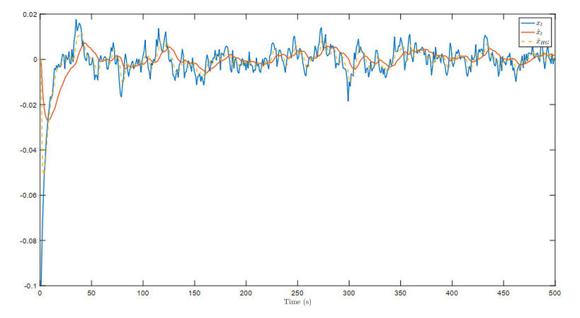
Figure 1. The estimation of the system state
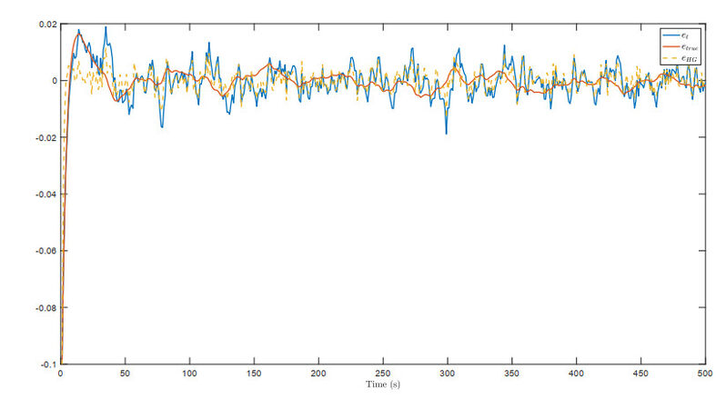
Figure 2. The estimation error of the system state
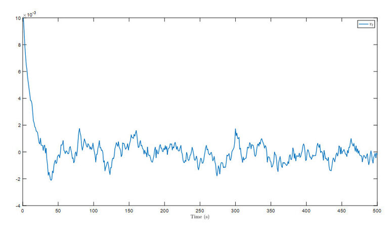
Figure 3. The compensative signal
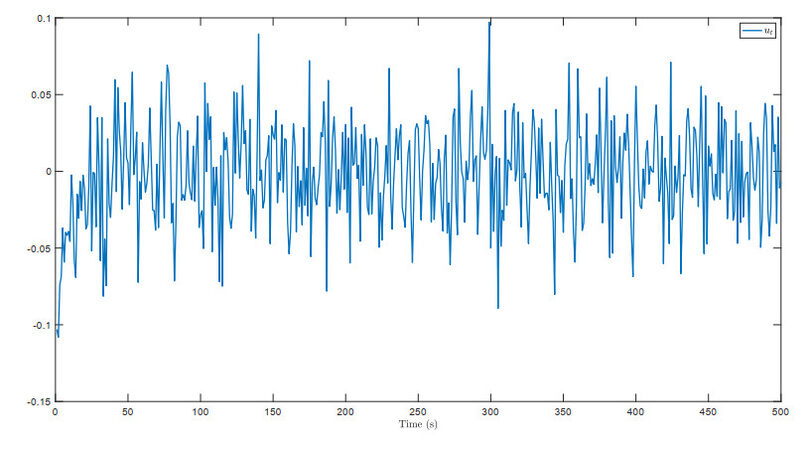
Figure 4. The compensative signal ut of filter before integral.
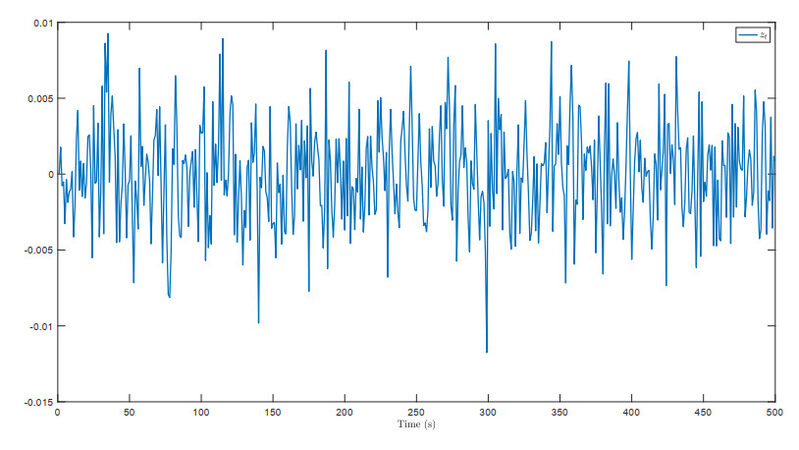
Figure 5. The trajectory of the virtual error
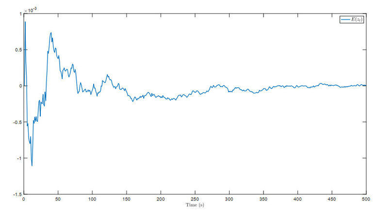
Figure 6. The mean value of the virtual error signal
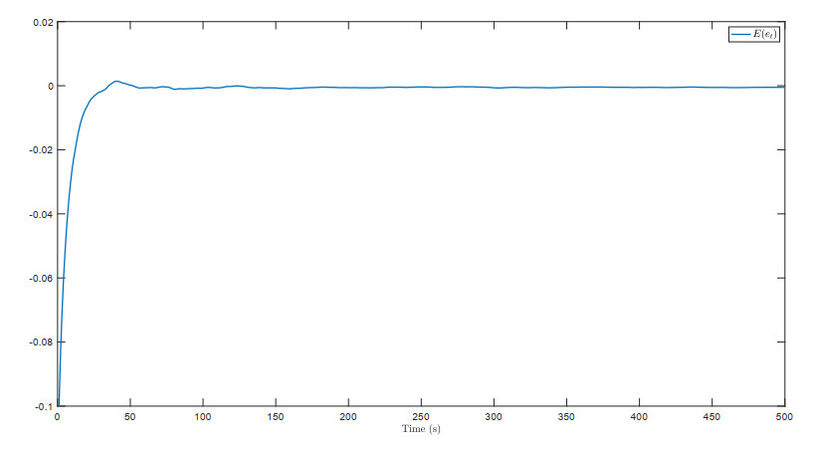
Figure 7. The mean value of the estimation error
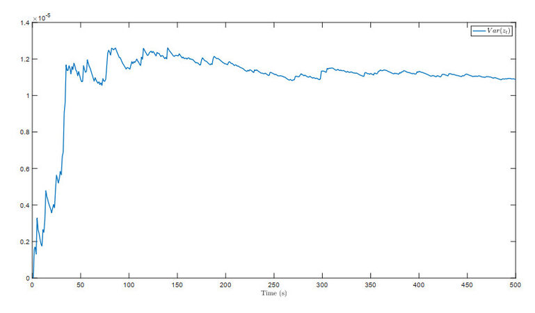
Figure 8. The variance of the virtual error signal
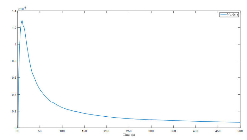
Figure 9. The variance of the estimation error
6. DISCUSSION
Only the single variable estimation is considered above to simplify the backstepping design. The main challenge of extending the presented algorithm to the multivariate case is basically the multi-variable backstepping design. Inspired by multi-variable controller design[23], the block backstepping design is one of the potential solutions. The system model in Equation (1) can be extended to vector-valued form as follows:
where
Then, the filter structure can be confirmed in vectorized form.
where
Similar to the design procedure, the Lyapunov functions can also be reused where the vector-value variables will be used. Since Lemma 2 holds for the multivariate system, the developed result in this paper can be extended directly following the block backstepping design. Notice that the linear Ornstein-Uhlenbeck process will be in the multi-dimensional form which leads to difficulty in solving the FPK equation as the joint probability density function has to be involved in the multivariate case. To avoid this problem, the design parameter
In addition, the measurement noise cannot be ignored in practice. An extended model should be formulated with the measurement noise which can be expressed as another stochastic differential equation. Thus, the convergence of the estimation error cannot be simply converted as the proposed linear dynamics. This extension will be considered as a future work with other assumptions.
7. CONCLUSION
The state estimation problem is investigated for a class of stochastic nonlinear systems, where the system model is described by the stochastic differential equation. To achieve the design objective, a new nonlinear filtering approach is designed. In particular, the design scheme is divided into two components: (1) The filtering structure can be confirmed based on the system model while the nonlinear estimation error can be further formulated. Then, an integrator is introduced into the estimation error for matching the backstepping design procedure. After that, the nonlinear dynamics can be converted to a linear Ornstein-Uhlenbeck process, where the mean value and variance value of the obtained estimation error is adjustable. (2) Since the variance value can be formulated analytically, the parameter can be designed for the filter. Ideally, the Brownian motion can be considered to obtain the desired variance value. Then, the design parameter in backstepping can be confirmed in order to attenuate the randomness of the state estimation. The simulation results and the multivariate system extension are also given to show the effectiveness and the potential extension of the presented estimation method. To extend the presented results, some comparative studies will be produced as future work where high-order sliding mode design[24, 25] and adaptive high-gain design[26] will be further considered.
DECLARATIONS
Acknowledgments
The authors would like to thank the reviewers for their valuable comments.
Authors' contributions
Made substantial contributions to conception and design of the study and performed data analysis and interpretation: Zhang Q
Performed data acquisition, as well as provided administrative, technical, and material support: Yin X
Availability of data and materials
Not applicable.
Financial support and sponsorship
None.
Conflicts of interest
Both authors declared that there are no conflicts of interest.
Ethical approval and consent to participate
Not applicable.
Consent for publication
Not applicable.
Copyright
© The Author(s) 2022.
REFERENCES
1. Barfoot TD. State estimation for robotics. Cambridge University Press; 2017.
2. Shukla N, Tiwari MK, Beydoun G. Next generation smart manufacturing and service systems using big data analytics. Elsevier; 2019.
3. Ben-Akiva M, Bierlaire M, Burton D, Koutsopoulos HN, Mishalani R. Network state estimation and prediction for real-time transportation management applications. In: Transportation Research Board 81st Annual Meeting; 2002.
4. Tang X, Zhang Q, Hu L. An EKF-based performance enhancement scheme for stochastic nonlinear systems by dynamic set-point adjustment. IEEE Access 2020;8:62261-72.
5. Zhou Y, Zhang Q, Wang H, Zhou P, Chai T. Ekf-based enhanced performance controller design for nonlinear stochastic systems. IEEE Transactions on Automatic Control 2017;63:1155-62.
6. Kalman RE. A new approach to linear filtering and prediction problems 1960.
7. Ribeiro MI. Kalman and extended kalman filters: Concept, derivation and properties. Institute for Systems and Robotics 2004;43:46.
8. Xiong K, Zhang H, Chan C. Performance evaluation of UKF-based nonlinear filtering. Automatica 2006;42:261-70.
9. Kalman RE, Bucy RS. New results in linear filtering and prediction theory 1961.
10. Xiao X, Xi H, Zhu J, Ji H. Robust Kalman filter of continuous-time Markov jump linear systems based on state estimation performance. International Journal of Systems Science 2008;39:9-16.
11. Sarkka S. On unscented Kalman filtering for state estimation of continuous-time nonlinear systems. IEEE Transactions on Automatic Control 2007;52:1631-41.
12. Djuric PM, Kotecha JH, Zhang J, Huang Y, Ghirmai T, et al. Particle filtering. IEEE signal processing magazine 2003;20:19-38.
13. Guo L, Wang H. Minimum entropy filtering for multivariate stochastic systems with non-Gaussian noises. IEEE Transactions on Automatic control 2006;51:695-700.
14. Zhang Q. Performance enhanced Kalman filter design for non-Gaussian stochastic systems with data-based minimum entropy optimisation. AIMS Electronics and Electrical Engineering 2019;3:382-96.
15. Ghoreyshi A, Sanger TD. A nonlinear stochastic filter for continuous-time state estimation. IEEE Transactions on Automatic Control 2015;60:2161-65.
16. Ross SM, Kelly JJ, Sullivan RJ, Perry WJ, Mercer D, et al. Stochastic processes. vol. 2. Wiley New York; 1996.
17. Zhang Q, Wang Z, Wang H. Parametric covariance assignment using a reduced-order closed-form covariance model. Systems Science & Control Engineering 2016;4:78-86.
18. Zhang Q, Wang H. A Novel Data-based Stochastic Distribution Control for Non-Gaussian Stochastic Systems. IEEE Transactions on Automatic Control 2021; doi: 10.1109/TAC.2021.3064991.
19. Zhang Q, Sepulveda F. A model study of the neural interaction via mutual coupling factor identification. In: 2017 39th Annual International Conference of the IEEE Engineering in Medicine and Biology Society (EMBC). IEEE; 2017. pp. 3329-32.
20. Zhang Q, Sepulveda F. A statistical description of pairwise interaction between nerve fibres. In: 2017 8th International IEEE/EMBS Conference on Neural Engineering (NER). IEEE; 2017. pp. 194-98.
21. Minskii R. Stochastic stability of differential equations, vol. 7 of Monographs and Textbooks on Mechanics of Solids and Fluids: Mechanics and Analysis. Sijthoff & Noordhoff, Alphen aan den Rijn 1980.
22. Liu SJ, Zhang JF, Jiang ZP. Decentralized adaptive output-feedback stabilization for large-scale stochastic nonlinear systems. Automatica 2007;43:238-51.
23. Zhang QC, Hu L, Gow J. Output feedback stabilization for MIMO semi-linear stochastic systems with transient optimisation. International Journal of Automation and Computing 2020;17:83-95.
24. Bejarano FJ, Fridman L. High order sliding mode observer for linear systems with unbounded unknown inputs. International Journal of Control 2010;83:1920-29.
25. Benallegue A, Mokhtari A, Fridman L. High-order sliding-mode observer for a quadrotor UAV. International Journal of Robust and Nonlinear Control: IFAC-Affiliated Journal 2008;18:427-40.
Cite This Article
Export citation file: BibTeX | RIS
OAE Style
Yin X, Zhang Q. Backstepping-based state estimation for a class of stochastic nonlinear systems. Complex Eng Syst 2022;2:1. http://dx.doi.org/10.20517/ces.2021.13
AMA Style
Yin X, Zhang Q. Backstepping-based state estimation for a class of stochastic nonlinear systems. Complex Engineering Systems. 2022; 2(1): 1. http://dx.doi.org/10.20517/ces.2021.13
Chicago/Turabian Style
Yin, Xin, Qichun Zhang. 2022. "Backstepping-based state estimation for a class of stochastic nonlinear systems" Complex Engineering Systems. 2, no.1: 1. http://dx.doi.org/10.20517/ces.2021.13
ACS Style
Yin, X.; Zhang Q. Backstepping-based state estimation for a class of stochastic nonlinear systems. Complex. Eng. Syst. 2022, 2, 1. http://dx.doi.org/10.20517/ces.2021.13
About This Article
Copyright

Data & Comments
Data


 Cite This Article 25 clicks

 Like This Article 16
likes
Like This Article 16
likes


Comments
Comments must be written in English. Spam, offensive content, impersonation, and private information will not be permitted. If any comment is reported and identified as inappropriate content by OAE staff, the comment will be removed without notice. If you have any queries or need any help, please contact us at support@oaepublish.com.