Research Article | Open Access | 30 Mar 2022

Comparison of battery modeling regression methods for application to unmanned aerial vehicles

Views: 1192 | Downloads: 604 | Cited:

Jon Ander Martin¹

, ...

Kelly Cohen¹

Complex Eng Syst 2022;2:5.

10.20517/ces.2022.03 | © The Author(s) 2022.

Author Information

Article Notes

Cite This Article

Abstract

An effective battery prognostics method is fundamental for any application in which batteries have a critical role, such as in unmanned aerial vehicles. Given the batteries' variable nature, effectively predicting their End of Discharge or End of Life can become a difficult task. Therefore, developing an accurate and efficient model becomes a key step of this problem. The framework provided by traditional modeling techniques usually leads to inaccurate results, so newer state-of-the-art methodologies are needed to successfully build a model from a dataset. This paper compares the accuracy and time performance of three existing methods: a maximum likelihood optimal Support Vector Machine, a Bayesian Relevance Vector Machine, and a Fuzzy Inference System. Through this research, we aim to implement a real-time battery prognostics system in an Unmanned Aerial Vehicle. The three methods are used to model a Lithium-ion (Li-ion) battery's discharge curve while accounting for the State of Health of the battery for the estimation of voltage. This paper compares the accuracy and time performance of a maximum likelihood optimal Support Vector Machine, a Bayesian Relevance Vector Machine, and a Fuzzy Inference System for the modeling of Lithium-ion (Li-ion) batteries' discharge curve. Moreover, the model accounts for the State of Health of the battery for the estimation of voltage. We show that the three methodologies are valid for the modeling of the discharge curve with similar accuracy values. The Relevance Vector Machine proves to be the most computationally efficient method.

Keywords

Optimization, fuzzy, bayesian, battery, unmanned aerial vehicle

Download PDF 0 42

1. INTRODUCTION

The electrical power system of an unmanned aerial vehicle (UAV) is one of the most critical subsystems in such aircraft. With advanced air mobility (AAM) poised as one of the future paradigms of civil aviation, these systems have been identified as key technologies for the successful integration of AAM ^[1]. Electrical Power systems, batteries, and emerging energy dense solutions are highlighted as technologies to be further developed and investigated for both safety as well as redundancy in the In-time Aviation Safety Management System report ^{[2, 3]}. Utilizing emerging artificial intelligence (AI) strategies to perform traditional pilot functions, such as predicting the state of health (SOH) of electrical systems, offers safety mechanisms and failsafes required before AAM reaches desired maturity levels ^{[1, 4]}.

An electrical power system is formed by several components, batteries being the most critical ^[4]. A failure in a battery can result in catastrophic failure of the entire vehicle. Therefore, it is essential to have reliable prognostics for a battery's end of discharge (EOD) and end of life (EOL). Further, it is also interesting to assess the confidence of the resulting prediction. The first step to solve such a problem is to have a reliable method to model the state of charge – voltage (SOC-V) curve depending on the SOH of the battery.

One of the problems we encounter when working with batteries is their variable nature. Their performance is strongly affected by environmental conditions, as well as its prior use cycles ^[5]. Therefore, modeling using traditional methods is a difficult task. One of the possible alternatives is to use data-driven methods, which utilize machine learning algorithms to establish battery degradation models ^{[6, 7]}. This approach allows the battery state estimation without a deep prior knowledge about the internal characteristics of the battery ^[8]. Examples of these methods are relevance vector machines (RVM), support vector machines (SVM), and Fuzzy Inference Systems (FIS). Model-based methods build a set of rules that model the behavior of the system ^[8]. Their main disadvantage is the need for a deep knowledge about the system and a lengthy amount of time to build the model. These methods often rely on internal parameters, which are inaccessible once a battery has been manufactured ^[9]. Therefore, they are not well suited for UAV applications.

Previous work proved an RVM and particle filter (PF) algorithm to be successful in the prediction of the remaining useful life (RUL), both for the state of charge (SOC) and SOH ^[10-12]. These methodologies have also been tested for their application in UAVs ^[13]. Other research has shown that the combination of RVM and SVM with sample entropy has been provided as a valid framework for battery prognostics ^[14]. Regarding fuzzy systems, previous research employed a fuzzy neural network for the estimation of the SOC with lithium iron phosphate batteries ^[15]. Work has also been done with respect to the SOH assessment using a FIS to combine the SOH assessment obtained from capacity measurements and internal resistance values ^[16]. Related to this matter, another fuzzy granulation methodology was tested to obtain a minimum and maximum boundary in the estimation of SOH by looking at the charging cycles ^[17]. Most of the work done with SVM regarding battery prognostics is aimed at the control of batteries ^{[18, 19]} or grid-scale battery storage models ^{[20, 21]}. Publications for this topic include SVM applied to SOH estimation ^[22] in combination with PF ^[23], fuzzy entropy ^[24], or incremental capacity analysis ^{[25, 26]}.

In this work we are comparing RVM, a Mamdani FIS and a maximum likelihood optimal SVM for the modeling of the SOC-V curves in batteries. We generate the battery discharge models with each methodology and then compare their accuracy and computational requirements. As mentioned above, this curve depends on the SOH: a battery with a lower SOH will show a faster decaying SOC-V curve. For convenience, we substitute the SOC with the state of discharge (SOD), which we define as $$ SOD = 1 - SOC $$ . We will include the current discharge cycle in the model as an estimation of the current SOH of the battery.

2. METHODS

In this section we present the SVM, RVM and FIS methodologies which were evaluated to solve the regression problem for a given dataset of battery discharge cycles. The general statement of the problem is as follows: obtain a function $$ f(\cdot) $$ from a labeled dataset $$ \left \{ \left( {\boldsymbol{x}}_s, y_s \right) \right \} ^N_{s=1} $$ .

2.1. Support vector regression with lncosh loss function

To calculate a regression with SVR, we map the input data into a high-dimensional feature space by using a kernel function $$ \varphi(\cdot): \mathbb{R}^n \rightarrow \mathbb{R}^m $$ and then perform a linear model

(1)

$$ \begin{equation} f\left({\boldsymbol{x}}, {\boldsymbol{w}}\right) = {\boldsymbol{w}}^T \varphi({\boldsymbol{x}}) + b \, , \end{equation} $$

where $$ {\boldsymbol{w}} \in \mathbb{R}^m $$ is the weight vector and $$ b $$ is the offset.

The success of SVR depends on the choice of the loss function, which represents the noise model of the dataset. This means that one must have some a priori information of the noise model in order to choose the proper loss function ^[27]. The so-called lncosh loss function we are using makes no assumptions about this noise model. Further, this function is convex and continuously differentiable. Thus, solving it with convex optimization techniques guarantees a globally optimal minimum ^[28].

The optimization problem to solve is

(2)

$$ \begin{equation} \min\limits_{{\boldsymbol{w}}, b} \left \{ \frac{1}{2} \| {\boldsymbol{w}} \|^2 + C \sum\limits_{s=1}^N \left[ l(\xi_s) + l(\xi^*_s) \right] \right \} , \end{equation} $$

subject to

(3)

$$ \begin{align} y_s - f({\boldsymbol{x}}_s, {\boldsymbol{w}}) &\leq \varepsilon + \xi_s \\ -y_s + f({\boldsymbol{x}}_s, {\boldsymbol{w}}) &\leq \varepsilon + \xi^*_s \\ \xi_s, \xi^*_s \geq 0&, \varepsilon \geq 0 \, , \end{align} $$

where

(4)

$$ \begin{equation} l(\xi_s) = lncosh_{\varepsilon} (\xi_s) = \begin{cases} 0 & \mbox{if } \lvert \xi_s \rvert < \varepsilon \\ \frac{1}{\lambda} \ln \left( \cosh_{\varepsilon} (\lambda \xi_s) \right) & \mbox{otherwise, } \end{cases} \end{equation} $$

$$ \xi_s $$ are independent random errors, $$ \varepsilon $$ is the size of the insensitive area, $$ C $$ is a parameter that determines the trade-off between flatness and empirical error, and $$ \lambda $$ is a parameter belonging to the lncosh function that controls the behavior of the loss function used ^[28].

Transformed using Lagrange multipliers, the dual-form problem is

(5)

$$ \begin{align} \min\limits_{{\boldsymbol{w}}, b, \alpha_s, \alpha_s^*, \gamma_s, \gamma_s^*, \xi_s, \xi_s^*} J = &\frac{1}{2} {\boldsymbol{w}}^T {\boldsymbol{w}} + C \sum\limits_{s=1}^N \left[ l(\xi_s) + l(\xi^*_s) \right] \\ &- \sum\limits_{s=1}^N \alpha_s \left( \varepsilon + \xi_s - y_s + {\boldsymbol{w}}^T\varphi({\boldsymbol{x}}_s) + b \right) \\ &- \sum\limits_{s=1}^N \alpha_s^* \left( \varepsilon + \xi_s^* + y_s - {\boldsymbol{w}}^T\varphi({\boldsymbol{x}}_s) - b \right) \\ &- \sum\limits_{s=1}^N \left( \gamma_s \xi_s + \gamma_s^* \xi_s^* \right) , \end{align} $$

where $$ \alpha_s, \alpha_s^*, \gamma_s, \gamma_s^* \geq 0 $$ are the Lagrange multipliers. Differentiating Equation (5) with respect to the primal variables $$ {\boldsymbol{w}}, b, \xi_s, \xi_s^* $$ and operating with the newly obtained equations yields the dual loss function

(6)

$$ \begin{align} \min\limits_{\alpha_s, \alpha_s^*} J = &\frac{1}{2} \left({\boldsymbol{\alpha}}-{\boldsymbol{\alpha}}^*\right)^T K \left({\boldsymbol{\alpha}}-{\boldsymbol{\alpha}}^*\right) \\ &+ \varepsilon \sum\limits_{s=1}^N \left( \alpha_s + \alpha_s^* \right) - {\boldsymbol{y}}^T \left({\boldsymbol{\alpha}}-{\boldsymbol{\alpha}}^*\right) \\ &- \frac{C}{\lambda} \sum\limits_{s=1}^N \left[ \ln \cosh_{\varepsilon} \left[{\rm{arctanh}}_{\varepsilon}\left(\frac{\alpha_s}{C}\right)\right] \right. \\ &- \frac{\alpha_s}{C} {\rm{arctanh}}_{\varepsilon}\left(\frac{\alpha_s}{C}\right) \\ &+ \ln \cosh_{\varepsilon} \left[{\rm{arctanh}}_{\varepsilon}\left(\frac{\alpha_s^*}{C}\right)\right] \\ &- \left. \frac{\alpha_s}{C} {\rm{arctanh}}_{\varepsilon}\left(\frac{\alpha_s^*}{C}\right)\right] \end{align} $$

that depends exclusively on the Lagrange multipliers $$ \alpha_s, \alpha_s^* $$ , where $$ {\boldsymbol{\alpha}}, {\boldsymbol{\alpha}}^* \in \mathbb{R}^N $$ are vectors containing the values of $$ \alpha_s, \alpha_s^* $$ , $$ K $$ is the kernel matrix with $$ K_{s, r} = \varphi^{T}({\boldsymbol{x}}_s) \cdot \varphi({\boldsymbol{x}}_r) $$ , and $$ {\boldsymbol{y}} \in \mathbb{R}^N $$ is a vector containing the values of $$ y_s $$ .

Equation (6) can be efficiently solved by an interior point optimization algorithm ^[29]. Once the values of $$ {\boldsymbol{\alpha}}, \, {\boldsymbol{\alpha}}^* $$ are known, the weights can be computed using

(7)

$$ \begin{equation} {\boldsymbol{w}} = \sum\limits_{s=1}^N \left( \alpha_s - \alpha_s^* \right) \varphi({\boldsymbol{x}}_s) \end{equation} $$

and the offset $$ b $$ is found with ^[30]

(8)

$$ \begin{equation} b = y_i - {\boldsymbol{w}}^T \varphi({\boldsymbol{x}}_i) - \varepsilon \mbox{ for } \alpha_i \in \left(0, C\right), \end{equation} $$

where $$ i $$ is picked from a multiplier $$ \alpha_i $$ that is not too close to $$ 0 $$ or $$ C $$ ^[31].

2.2. Relevance vector machine

RVM provides a probabilistic approach to the regression problem ^[32]. The method is similar to SVR in that it maps the inputs to a high-dimensional feature space and then computes a linear combination of weights with certain kernel functions

(9)

$$ \begin{equation} f\left({\boldsymbol{x}}, {\boldsymbol{w}}\right) = \sum\limits_{m=0}^M w_m \varphi(x, x_m) \, , \end{equation} $$

where $$ M $$ is the number of kernels used and $$ w_m $$ is the weight of kernel $$ m $$ .

For a pair of input and target $$ \left \{ \left( {\boldsymbol{x}}_s, y_s \right) \right \} ^N_{s=1} $$ , it is assumed they follow a Gaussian distribution of mean $$ f\left({\boldsymbol{x}}, {\boldsymbol{w}}\right) $$ and variance $$ \sigma^2 $$ . Therefore, the Gaussian function will depend on the weights. To prevent overfitting, a prior distribution is set over the weights

(10)

$$ \begin{equation} p\left({\boldsymbol{w}}\lvert{\boldsymbol{\alpha}}\right) = \prod\limits_{i=0}^M N\left(w_i\lvert 0, \alpha_i^{-1}\right) , \end{equation} $$

where $$ {\boldsymbol{w}} \in \mathbb{R}^M $$ is the weight vector and $$ {\boldsymbol{\alpha}}=\left(\alpha_1, \alpha_2, \ldots, \alpha_M\right)^T $$ is a vector with an individual hyperparameter for each of the weights. This prior distribution, with mean zero, makes the weights have low values, which benefits sparsity ^[33]. The complete process to build a model using RVM was described in detail by Fletcher ^[34].

2.3. Fuzzy Inference System

Fuzzy logic was proposed in 1965 by Zadeh ^[35]. It distinguishes from other methodologies in two key concepts. The first is the use of linguistic variables, i.e., variables whose content are words instead of numbers. This concept allows for a granulation of the input and output data. The second concept is the use of if-then linguistic rules ^[36]. Overall, the usage of variables close to natural language provides a comprehensible and explainable approach for humans ^[37]. Moreover, explainability can become an essential matter in airborne systems ^[38]. Other AI algorithms are essentially black boxes with complex decision systems. This can be an issue for certification organizations, since the inability to understand the insights of the decision-making process can reduce the trust that end users have on any system. Therefore, a FIS introduces a significant advantage with respect to other AI methodologies.

The FIS used for this work is a Mamdani-type FIS. In early trials of this work a Takagi-Sugeno algorithm was tested, but its training took longer and its performance was worse than Mamdani's dut to the difficulty choosing initial model parameters and the genetic algorithm (GA) tuning processing used for the FIS, so it was discarded. A Mamdani algorithm is characterized by fuzzy if-then rules with linguistic variables both in the input and output variables. For example, a rule takes the form of

(11)

$$ \begin{equation} \mbox{if } x \mbox{ is } A \mbox{ and } y \mbox{ is } B, \;{\rm{ then }}\; z \;{\rm{ is }}\; C \, , \end{equation} $$

where $$ x, y, z $$ are input or output variables and $$ A, B, C $$ are fuzzy subsets of those variables. In a 2-input 1-output system, as the one showed in Equation (11), we can compute a membership function $$ \mu_i $$ for every input with a triangular function given the left $$ l $$ , right $$ r $$ , and center $$ c $$ points with

(12)

$$ \begin{equation} \mu_i = \begin{cases} \frac{x_i-l}{c-l} & {\rm{if }}\; x_i \geq l \;{\rm{ and }}\; x_i < c \\ \frac{r-x_i}{r-c} & {\rm{if }}\; x_i \geq c \;{\rm{ and }}\; x_i < r \\ 0 & {\rm{otherwise}} . \end{cases} \end{equation} $$

The membership functions make some rules fire that yield degrees of membership in the output membership functions. In order to defuzzify these membership functions and produce a numerical value in the output, we use the centroid method, selected as it is continuous, monotonic, scale invariant, and well known ^{[39, 40]}. This method aggregates the membership functions of the output variables and computes the center of gravity of them. The equation used is

(13)

$$ \begin{equation} z = \frac{\int_{a}^{b} x \mu_A(x) dx }{ \int_{a}^{b} \mu_A(x) dx } \, , \end{equation} $$

where $$ z $$ is the numerical output, $$ a, b $$ are the limits of the output range, and $$ \mu_A $$ is the aggregated membership function calculated according to the set of rules.

3. RESULTS

This section compares the battery discharge models obtained with the three algorithms. All of the models consist of 2 inputs (SOD and discharge cycle) and 1 output (battery voltage). The data utilized comes from the well-known Li-ion battery dataset provided by the NASA Ames Research Center ^[41]. The entire process is depicted in Figure 1. The results were obtained using MATLAB 2016a (lncosh-SVM and RVM) and Python 3.9.7 (fuzzy-GA) programming environments on a Windows 10 PC with an Intel Core i7-6000 processor at 3 GHz.

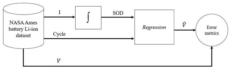
Comparison of battery modeling regression methods for application to unmanned aerial vehicles

Figure 1. Data flowchart of the process. $$ I $$ stands for current and $$ SOD $$ stands for State of Discharge. The integral symbol represents the Coulomb counting method, which integrates current to obtain the SOD. $$ V $$ is the labeled voltage and $$ \hat{V} $$ is the estimated voltage.

The parameters for the RVM algorithm were directly obtained from previous work ^[13]. The radii used for the radial basis functions (RBF) are $$ \sigma_1=60 $$ , $$ \sigma_2=500 $$ , $$ \sigma_3=1700 $$ , $$ \sigma_4=3400 $$ , and $$ \sigma_5=6800 $$ .

The user specified parameters in the SVM methodology can have a great impact on the results ^[42]. The initial parameters for the lncosh-SVM algorithm were obtained using our prior knowledge about the system from the RVM algorithm. The values were further optimized using a GA. GAs are a set of population-based stochastic algorithms that mimic the process of natural evolution to optimize a given function ^[43]. The parameters obtained after this process were $$ \lambda = 1083 $$ , $$ \varepsilon = 0.0153 $$ and $$ C = 0.00612 $$ . The value obtained for $$ \lambda $$ suggests that the lncosh loss function will behave in a similar way to $$ \varepsilon $$ -insensitive Huber's loss. We decided to use 5 RBF as kernels, in the same way we did with RVM. Their radii were also optimized using the GA, their final values being $$ \sigma_1=92 $$ , $$ \sigma_2=649 $$ , $$ \sigma_3=1631 $$ , $$ \sigma_4=2863 $$ , and $$ \sigma_5=5619 $$ .

The rule base and the initial membership function values of the FIS are manually set based on expert knowledge and previous experience with the topic. The membership functions, as shown in Equation (12), are all triangular. Further, with the aim of simplifying the learning process, all the triangles are isosceles. These triangles are handcrafted based on prior knowledge as an initial approximation and then further optimized using a GA ^{[44, 45]}. We use 3 membership functions for each input variable, and 5 membership functions for the output value. In the GA learning process, we encode the centers and base widths of all the triangular membership functions, giving a total of 22 genes per chromosome. The error function compares and minimizes the absolute value of the difference between the labeled values and the results obtained with the FIS, i.e., $$ e = \lvert \hat{y}_s - y_s \rvert $$ . The genetic operators used are roulette-wheel selection, single point crossover, Gaussian mutation and elitism. The optimization process runs for a fixed number of 350 generations. The parameters for the genetic operators and the number of generations were chosen based on preliminary runs of the algorithm. This GA utilizes parallel processing, with 10 workers computing the fitness value of 10 chromosomes simultaneously.

The NASA Ames Research Center dataset provides 3 different battery discharge cycle datasets named: B0005, B0006 and B0007. We have tested the 3 methodologies with each of these discharge cycle datasets. Figures 2-4 show the regressions obtained with the 3 methodologies being tested. All the figures presented have been obtained from the dataset B0005. For each of the discharge cycle datasets, a 5-fold cross validation technique is used. Therefore, the experiments are repeated 15 times per algorithm. The results obtained with each discharge cycle dataset are then averaged and displayed in Tables 1-3. The metrics used for the comparison are the Root Mean Squared Error (RMSE) defined as

(14)

$$ \begin{equation} \mbox{RMSE} = \sqrt{\sum\limits_{s=1}^N \frac{\left(\hat{y}_s - y_s\right)^2}{N}} \end{equation} $$

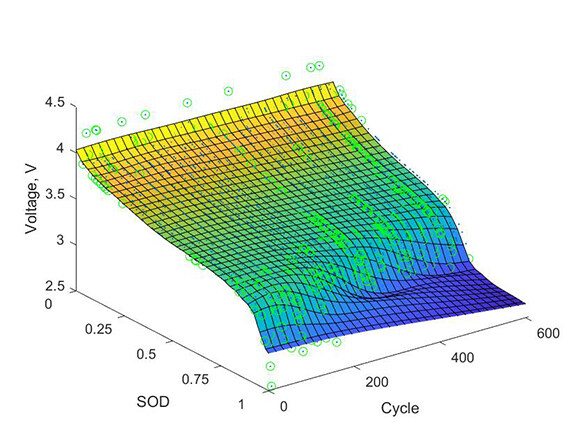
Figure 2. Comparison between SVM regression and datapoints. The surface represents the SVM regression. The datapoints used as Support Vectors are highlighted in green. SVM: support vector machin; SOD: state of discharge. The cycle is the number of times the battery has been charged and discharged throughout its lifetime.

Figure 3. Comparison between RVM regression and datapoints. The surface represents the RVM regression. RVM: relevance vector machine; SOD: state of discharge. The cycle is the number of times the battery has been charged and discharged throughout its lifetime.

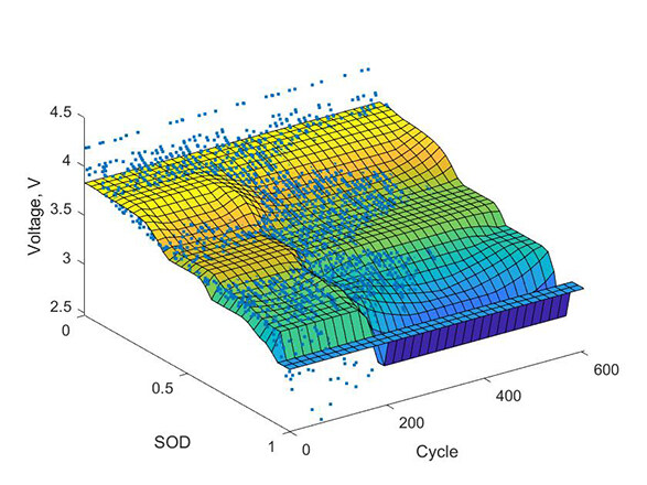
Figure 4. Comparison between FIS regression and datapoints. The surface represents the FIS regression. FIS: Fuzzy Inference System; SOD: state of discharge. The cycle is the number of times the battery has been charged and discharged throughout its lifetime.

Table 1

Comparison of results with dataset B0005

Methodology	RMSE	MAE	$$ \\| {\boldsymbol{w}} \\|^2 $$ ^a	#Relevance/support vectors^b	Training time^c (min)
^a$$ \\| {\boldsymbol{w}} \\|^2 $$ is the norm of the weights of the model in SVM and RVM, and represents a measure of the flatness of the solution. ^bNumber of Relevance Vectors in the case of RVM, number of Suppor Vectors in the case of lncosh-SVM. These concepts are equivalent in these methodologies. ^cThe training time is the total time needed to build the regression model with each methodology. In lncosh-SVM this means solving Equation (6) and then computing the weights with Equation (7). In RVM the weights in Equation (9) are found using the iterative process described by Fletcher ^[34]. In Fuzzy-GA it refers to the time needed to run the GA that optimizes the membership functions.
lncosh-SVM	0.0711	0.0551	0.0466	386.2	141.7
RVM	0.0708	0.0676	10142	50.2	1.2
Fuzzy-GA	0.0894	0.0560	-	-	98.3

Table 2

Comparison of results with dataset B0006^a

Methodology	RMSE	MAE	$$ \\| {\boldsymbol{w}} \\|^2 $$	#Relevance/Support vectors	Training time (min)
^aSee footnotesin Table 1.
lncosh-SVM	0.1136	0.0898	0.0604	749.4	137.6
RVM	0.1307	0.1317	194961	63.0	1.2
Fuzzy-GA	0.1068	0.0626	-	-	100.4

Table 3

Comparison of results with dataset B0007^a

Methodology	RMSE	MAE	$$ \\| {\boldsymbol{w}} \\|^2 $$	#Relevance/Support vectors	Training time (min)
^aSee footnotesin Table 1.
lncosh-SVM	0.1195	0.0662	0.0647	1137.6	150.4
RVM	0.1107	0.0859	1051199	74.2	1.1
Fuzzy-GA	0.1234	0.0585	-	-	97.7

and Mean Absolute Error (MAE) defined as

(15)

$$ \begin{equation} \mbox{MAE} = \frac{1}{N} \sum\limits_{s=1}^N \lvert \hat{y}_s - y_s \rvert \, . \end{equation} $$

There is no clear best method in terms of accuracy. The results vary across datasets and they depend on what error metric we consider. Looking at the results obtained from B0005, lncosh-SVM's RMSE is 0.4% higher than RVM's, but the MAE is 22.7% lower. The lncosh-SVM outperforms the FIS with 25.7% and 1.6% decreases in RMSE and MAE, respectively. In dataset B0006, the RMSE of lncosh-SVM is 15.1% lower than the one provided by RVM and the MAE 46.7% lower. However, the FIS is the methodology with the best accuracy in this case. The results show a 5.9% reduction in RMSE and 30.3% reduction in MAE with respect to lncosh-SVM. In B0007, the lncosh-SVM methodology shows a 7.4% increase in RMSE with respect to RVM, but lncosh-SVM provides a 29.8% decrease in MAE compared to RVM. The FIS shows a RMSE 3.3% higher than lncosh-SVM's. However, its MAE is 11.6% lower.

The values of $$ \| {\boldsymbol{w}} \|^2 $$ are shown as a measure of flatness and sparsity of the solution. The lncosh-SVM has much lower values than RVM, which means that the RBF that compose the solution are smoother in the case of lncosh-SVM. This fact can also be observed in Figures 2 and 3. However, it is worth noting that the very high values in RVM are heavily influenced by a single very high result in one of the runs of the 5-fold cross validation process, which skews the average score. This phenomenon happened with all the discharge cycle datasets.

In terms of computation time, RVM is the most efficient method by a big difference. Its training takes about a minute to complete, while lncosh-SVM and the FIS need between 1 and 3 hours to complete the training process. This fact is supported by the difference in the number of support or relevance vectors: RVM needs, on average, 7.7 times less support vectors in B0005, 11.9 in B0006 and 15.3 in B0007. As a consequence, an RVM model requires less memory capacity, which can be crucial for applications where less capable single-board computers are used, such as for UAVs ^[46].

4. DISCUSSION

This study compares the accuracy and computational cost when modeling a battery discharge cycle with lncosh-SVM, RVM and a FIS. A successful prediction of the EOD and EOL of batteries and an assessment of its uncertainty is essential for the safe operation of UAV. The methodologies tested provide a framework to model the SOD – V curve and incorporate a measure of the SOH to account for the natural variability of batteries along their lifetime. To fully predict the EOD of the battery and the remaining flight time of a UAV, these regression techniques can be combined with a prediction methodology, such as a Kalman filter or PF, which should be further explored as an extension to this work.

The results presented show that the 3 methodologies could be used to solve this problem at varying computational costs. The lncosh-SVM shows the best accuracy in most cases, but at a high computational cost. RVM is able to yield results within a 15.1% RMSE and 46.7% MAE at a much lower computational cost. The FIS has, in general, the worst performance in RMSE, but can improve on the lncosh-SVM MAE provided by up to 30.3%. Its computational cost lies in between the other two methods.

We did not anticipate these results, specially those obtained with the FIS. The lncosh-SVM, being maximum likelihood optimal, was expected to show the best results in terms of accuracy. Since RVM is a probabilistic approach, but similar in nature, we were expecting to see small increases in its error metrics when compared to lncosh-SVM. The FIS was expected to have the lowest accuracies of the three options. However, the results show that it can have accuracies similar to lncosh-SVM's and RVM's, and even improve them in some cases. A significant advantage of the FIS that contributes to making it an attractive method is that it allows the system to be more explainable and comprehensible, relevant features toward certification of airborne systems.

As previously stated, Matlab 2016a was used to obtain the results from lncosh-SVM and RVM, while Python 3.9.7 was used to obtain the results of the fuzzy-GA methodology. Using different programming languages could affect the accuracy of the comparison between training times. However, the training times presented in Tables 1-3 for the three methodologies are so distinct from each other that we believe this is enough evidence to classify RVM as the fastest method, with fuzzy-GA being second and lncosh-SVM third. In the future, it could be interesting to compare these methodologies using exclusively Python. This language is more appropriate in applications such as UAVs, where single-board computers are often used. The results of such an experiment could be decisive to favor one methodology over the others in this particular application.

Further, one could also argue that the GA itself could be further optimized for faster performance or to yield more optimal results. Figure 4 shows that the FIS divides the discharge into three regions with a distinct valley in the middle of the discharge and steep decreases in between. It is an interesting result to observe, specifically when compared to Figures 2 and 3, where the regressions are smoother. This could be interpreted as a feature that the FIS extracted from the data or as a possibility of further improvement of the GA and FIS in general. The parameters of the GA were tuned to the best of our knowledge using research and previous experience. For performance comparisons of our methods and models, we assume that the GA used performs at its highest level. Future work could be directed at further analyzing this algorithm to improve its performance and convergence time for this particular application. However, other studies have shown that when tuning GA control parameters, good performance can be obtained with a range of GA control parameter settings ^{[47, 48]}. We can therefore expect only little improvement after many trials with different GA parameter sets.

Another limitation of the results shown comes from the dataset itself. The data was obtained in controlled experiments in a lab. Therefore, this data does not account for inaccuracies, measurement errors or external noise, as with with UAVs subject to external factors. Future work will compare these same methodologies using battery discharge data obtained through hardware analysis using an Orion Jr. 2 Battery Management System as payload onboard a UAV. This will allow us to evaluate the results with new raw datasets coming directly from the target of our research.

5. CONCLUSIONS

AAM is one of the future paradigms of civil aviation and the use of AI offers an opportunity to fundamentally substitute, alter, or augment the traditional pilot functions. Batteries have been identified as critical subsystems in an electric UAV because their variable nature and dependence on prior usage makes their modeling difficult. This paper investigates the application of SVM, RVM, and FIS to model a battery's discharge curve. We show how to apply the three methodologies while accounting for the SOH of the battery in the moment of the discharge. The results prove that the three methodologies provide useful frameworks to solve the problem. SVM shows the best accuracy in most cases, but at a high computational cost. RVM can provide results similar in accuracy at a much lower computational cost. The FIS is able to improve the MAE of the other methodologies, with an intermediate computational cost. In future steps of this research we will implement the outline methodologies on-board an electric UAV and apply them in a real-time manner.

DECLARATIONS

Authors' contributions

Concept development: Martin J, Ouwerkerk JN, Lamping AP, Cohen K

Manuscript drafting: Martin J

Manuscript edition and review: Ouwerkerk JN, Lamping AP, Cohen K

Availability of data and materials

The dataset used for this work was created by the NASA Ames Research Center and is publicly available at https://c3.ndc.nasa.gov/dashlink/resources/133.

Financial support and sponsorship

None.

Conflicts of interest

All authors declared that there are no conflicts of interest.

Ethical approval and consent to participate

Not applicable.

Consent for publication

Not applicable.

Copyright

REFERENCES

1. NASA/Deloitte Consulting LLP. UAM Vision Concept of Operations (ConOps) UAM Maturity Level (UML) 4. NASA; 2021. Available from: https://www.nasa.gov/aeroresearch/uam-vision-conops-uml-4[Last accessed on 23 Mar 2022].

2. Johnson W, Silva C. NASA concept vehicles and the engineering of advanced air mobility aircraft. Aeronaut J 2022;126:59-91.

3. Ellis KK, Krois P, Koelling JH, Prinzel LJ, Davies MD, Mah RW. Defining services, functions, and capabilities for an Advanced Air Mobility (AAM) In-time Aviation Safety Management System (IASMS). AIAA Aviation 2021 Forum: Proceedings of the AIAA Aviation 2021 Forum; 2021; pp. 2396.

4. Desai K, Al Haddad C, Antoniou C. Roadmap to early implementation of passenger air mobility: findings from a delphi study. Sustainability 2021;13:10612.

5. Warren M, Garbo A, Herniczek MTK, Hamilton T, German B. Effects of range requirements and battery technology on electric VTOL sizing and operational performance. AIAA Scitech 2019 Forum: Proceedings of the AIAA Scitech 2019 Forum; 2019; pp. 0527.

6. Li X, Yuan C, Wang Z. Multi-time-scale framework for prognostic health condition of lithium battery using modified Gaussian process regression and nonlinear regression. J Power Sources 2020;467:228358.

7. Wang S, Fernandez C, Yu C, Fan Y, Cao W, et al. A novel charged state prediction method of the lithium ion battery packs based on the composite equivalent modeling and improved splice Kalman filtering algorithm. J Power Sources 2020;471:228450.

8. How DNT, Hannan MA, Hossain Lipu MS, Ker PJ. State of charge estimation for lithium-ion batteries using model-based and data-driven methods: a review. IEEE Access 2019;7:136116-36.

9. Feng Y, Xue C, Han QL, Han F, Du J. Robust Estimation for State-of-Charge and State-of-Health of Lithium-Ion Batteries Using Integral-Type Terminal Sliding-Mode Observers. IEEE T Ind Electron 2020;67:4013-23.

10. Saha B, Goebel K, Poll S, Christophersen J. Prognostics methods for battery health monitoring using a bayesian framework. IEEE T Instrum Meas 2009;58:291-96.

11. Goebel K, Saha B, Saxena A, Celaya JR, Christophersen JP. Prognostics in battery health management. IEEE Instru Meas Mag 2008;11:33-40.

12. Mo B, Yu J, Tang D, Liu H, Yu J. A remaining useful life prediction approach for lithium-ion batteries using Kalman filter and an improved particle filter. 2016 IEEE International Conference on Prognostics and Health Management (ICPHM): Proceedings of the 2016 IEEE International Conference on Prognostics and Health Management; 2016. pp. 1-5.

13. Martin JA, Ouwerkerk JN, Lamping AP, Cohen K. Relevance vector machine and particle filter for unmanned aerial vehicle battery prognostics. AIAA Scitech 2021 Forum: Proceedings of the AIAA Scitech 2021 Forum; 2021.

14. Widodo A, Shim MC, Caesarendra W, Yang BS. Intelligent prognostics for battery health monitoring based on sample entropy. Expert Syst Appl 2011;38:11763-69.

15. Song S, Wei Z, Xia H, Cen M, Cai C. State-of-charge (SOC) estimation using T-S fuzzy neural network for lithium iron phosphate battery. 2018 26th International Conference on Systems Engineering (ICSEng): Proceedings of the 2018 26th International Conference on Systems Engineering; 2018; pp. 1-5.

16. Ananto P, Syabani F, Indra WD, Wahyunggoro O, Cahyadi AI. The state of health of Li-Po batteries based on the battery's parameters and a fuzzy logic system. 2013 Joint International Conference on Rural Information Communication Technology and Electric-Vehicle Technology (rICT ICeV-T): Proceedings of the 2013 Joint International Conference on Rural Information Communication Technology and Electric-Vehicle Technology; 2013. pp. 1-4.

17. Pan W, Chen Q, Zhu M, Tang JL, Wang J. A data-driven fuzzy information granulation approach for battery state of health forecasting. J Power Sources 2020;475:228716.

18. Khamar M, Askari J. A charging method for Lithium-ion battery using Min-max optimal control. 2014 22nd Iranian Conference on Electrical Engineering (ICEE): Proceedings of the 2014 22nd Iranian Conference on Electrical Engineering; 2014; pp. 1239-43.

19. Rashid A, Hofman T, Rosca B. Enhanced battery thermal management systems with optimal charge control for electric vehicles. 2018 Annual American Control Conference (ACC): Proceedings of the 2018 Annual American Control Conference; 2018; pp. 1849-54.

20. Rosewater DM, Copp DA, Nguyen TA, Byrne RH, Santoso S. Battery energy storage models for optimal control. IEEE Access 2019;7:178357-91.

21. Wu D, Balducci PJ, Crawford AJ, Viswanathan VV, Kintner-Meyer MC. Optimal control for battery storage using nonlinear models; 2018, 1. Available from: https://www.osti.gov/biblio/1647339[Last accessed on 23 Mar 2022].

22. Patil MA, Tagade P, Hariharan KS, Kolake SM, Song T, et al. A novel multistage Support Vector Machine based approach for Li ion battery remaining useful life estimation. Appl Energ 2015;159:285-97.

23. Wei J, Dong G, Chen Z. Remaining useful life prediction and state of health diagnosis for lithium-ion batteries using particle filter and support vector regression. IEEE T Ind Electron 2018;65:5634-43.

24. Sui X, He S, Stroe DI, Teodorescu R. State of Health estimation for lithium-ion battery using fuzzy entropy and support vector machine. 2020 IEEE 9th International Power Electronics and Motion Control Conference (IPEMC2020-ECCE Asia): Proceedings of the 2020 IEEE 9th International Power Electronics and Motion Control Conference; 2020; pp. 1417-22.

25. Vatani M, Szerepko M, Preben Vie JS. State of health prediction of Li-ion batteries using incremental capacity analysis and support vector regression. 2019 IEEE Milan PowerTech: Proceedings of the 2019 IEEE Milan PowerTech conference; 2019; pp. 1-6.

26. Li L, Cui W, Hu X, Chen Z. A state-of-health estimation method of lithium-ion batteries using ICA and SVM. 2021 Global Reliability and Prognostics and Health Management (PHM-Nanjing): Proceedings of the 2021 Global Reliability and Prognostics and Health Management conference; 2021; pp. 1-5.

27. Huber PJ. Robust estimation of a location parameter. Ann Math Stat 1964;35:73-101.

28. Karal O. Maximum likelihood optimal and robust Support Vector Regression with lncosh loss function. Neural Networks 2017;94:1-12.

29. Smola AJ, Schölkopf B, Müller KR. General cost functions for support vector regression. 8th International Conference on Artificial Neural Networks: Proceedings of the 8th International Conference on Artificial Neural Networks; 1998; pp. 79-83. Available from: http://citeseerx.ist.psu.edu/viewdoc/summary?doi=10.1.1.41.2760[Last accessed on 23 Mar 2022].

30. Awad M, Khanna R. Efficient learning machines: theories, concepts, and applications for engineers and system designers. In: Support Vector Regression. Berkeley, CA: Apress; 2015. pp. 67-80.

31. Schölkopf B, Smola AJ. Learning with kernels: support vector machines, regularization, optimization, and beyond. Boston, MA: The MIT Press; 2018.

32. Tipping M. Advances in Neural Information Processing Systems. vol. 12. In: Solla S, Leen T, Müller K, editors. The Relevance Vector Machine. Boston, MA: The MIT Press; 2000. pp. 652-58. Available from: https://proceedings.neurips.cc/paper/1999/file/f3144cefe89a60d6a1afaf7859c5076b-Paper.pdf [Last accessed on 23 Mar 2022].

33. Tipping ME. Sparse bayesian learning and the relevance vector machine. J Mach Learn Res 2001 9;1: 211-44.

34. Fletcher T. Relevance Vector Machines Explained. London's Global University 2010, 10. Available from: https://static1.squarespace.com/static/58851af9ebbd1a30e98fb283/t/58902f4a6b8f5ba2ed9d3bfe/1485844299331/RVM+Explained.pdf[Last accessed on 23 Mar 2022].

35. Zadeh LA. Fuzzy sets. Inform Control 1965;8:338-53.

36. Zadeh LA. Soft computing and fuzzy logic. IEEE Software 1994;11:48-56.

37. Fernández A, Herrera F, Cordón O, José del Jesús M, Marcelloni F. Evolutionary fuzzy systems for explainable artificial intelligence: why, when, what for, and where to? IEEE Comput Intell M 2019;14:69-81.

38. Saraf AP, Chan K, Popish M, Browder J, Schade J. Explainable artificial intelligence for aviation safety applications. AIAA Aviation 2020 Forum: Proceedings of the AIAA Aviation 2020 Forum; 2020.

39. Leekwijck WV, Kerre EE. Defuzzification: criteria and classification. Fuzzy Set Syst 1999;108:159-78.

40. Runkler TA. Selection of appropriate defuzzification methods using application specific properties. IEEE T Fuzzy Syst 1997;5:72-79.

41. NASA Ames Research Center. Li-ion Battery Aging Datasets; 2010. Available from: https://c3.ndc.nasa.gov/dashlink/resources/133[Last accessed on 23 Mar 2022].

42. Cherkassky V, Ma Y. Practical selection of SVM parameters and noise estimation for SVM regression. Neural Networks 2004;17:113-26.

43. Mirjalili S. Evolutionary algorithms and neural networks. New York City, NY: Springer International Publishing; 2019; pp. 43-55.

44. Buckley JJ, Hayashi Y. Fuzzy genetic algorithm and applications. Fuzzy Set Syst 1994;61:129-36.

45. Cordón O, Herrera F, Hoffmann F, Magdalena L. Genetic Fuzzy Systems. Singapore: World Scientific; 2001.

46. Lamping AP, Ouwerkerk JN, Cohen K. Multi-UAV Control and Supervision with ROS. 2018 Aviation technology, integration, and operations conference: Proceedings of the 2018 Aviation technology, integration, and operations conference; 2018. p. 4245.

47. Grefenstette JJ. Optimization of Control Parameters for Genetic Algorithms. IEEE T Syst Man Cyb 1986;16:122-28.

48. Schaffer JD, Caruana RA, Eshelman LJ, Das R. A Study of Control Parameters Affecting Online Performance of Genetic Algorithms for Function Optimization. Third International Conference on Genetic Algorithms: Proceedings of the Third International Conference on Genetic Algorithms. San Francisco, CA, USA: Morgan Kaufmann Publishers Inc.; 1989. pp. 51-60.

Cite This Article

Export citation file: BibTeX | RIS

OAE Style

Martin JA, Ouwerkerk JN, Lamping AP, Cohen K. Comparison of battery modeling regression methods for application to unmanned aerial vehicles. Complex Eng Syst 2022;2:5. http://dx.doi.org/10.20517/ces.2022.03

AMA Style

Martin JA, Ouwerkerk JN, Lamping AP, Cohen K. Comparison of battery modeling regression methods for application to unmanned aerial vehicles. Complex Engineering Systems. 2022; 2(1): 5. http://dx.doi.org/10.20517/ces.2022.03

Chicago/Turabian Style

Martin, Jon Ander, Justin N. Ouwerkerk, Anthony P. Lamping, Kelly Cohen. 2022. "Comparison of battery modeling regression methods for application to unmanned aerial vehicles" Complex Engineering Systems. 2, no.1: 5. http://dx.doi.org/10.20517/ces.2022.03

ACS Style

Martin, JA.; Ouwerkerk JN.; Lamping AP.; Cohen K. Comparison of battery modeling regression methods for application to unmanned aerial vehicles. Complex. Eng. Syst. 2022, 2, 5. http://dx.doi.org/10.20517/ces.2022.03

About This Article

Copyright

© The Author(s) 2022. Open Access This article is licensed under a Creative Commons Attribution 4.0 International License (https://creativecommons.org/licenses/by/4.0/), which permits unrestricted use, sharing, adaptation, distribution and reproduction in any medium or format, for any purpose, even commercially, as long as you give appropriate credit to the original author(s) and the source, provide a link to the Creative Commons license, and indicate if changes were made.

Data & Comments

Data

Views

1192

Downloads

604

Citations

Comments

Comments

Comments must be written in English. Spam, offensive content, impersonation, and private information will not be permitted. If any comment is reported and identified as inappropriate content by OAE staff, the comment will be removed without notice. If you have any queries or need any help, please contact us at support@oaepublish.com.