
A comparative study of energy management systems under connected driving: cooperative car-following case

Abstract
In this work, we propose connected energy management systems for a cooperative hybrid electric vehicle (HEV) platoon. To this end, cooperative driving scenarios are established under different car-following behavior models using connected and automated vehicles technology, leading to a cooperative cruise control system (CACC) that explores the energy-saving potentials of HEVs. As a real-time energy management control, an equivalent consumption minimization strategy (ECMS) is utilized, wherein global energy-saving is achieved to promote environment-friendly mobility. The HEVs cooperatively communicate and exchange state information and control decisions with each other by sixth-generation vehicle-to-everything (6G-V2X) communications. In this study, three different car-following behavior models are used: intelligent driver model (IDM), Gazis–Herman–Rothery (GHR) model, and optimal velocity model (OVM). Adopting cooperative driving of six Toyota Prius HEV platoon scenarios, simulations under New European Driving Cycle (NEDC), Worldwide Harmonized Light Vehicle Test Procedure (WLTP), and Highway Fuel Economy Test (HWFET), as well as human-in-the-loop (HIL) experiments, are carried out via MATLAB/Simulink/dSPACE for cooperative HEV platooning control via different car-following-linked-vehicle scenarios. The CACC-ECMS scheme is assessed for HEV energy management via 6G-V2X broadcasting, and it is found that the proposed strategy exhibits improvements in vehicular driving performance. The IDM-based CACC-ECMS is an energy-efficient strategy for the platoon that saves: (i) 8.29% fuel compared to the GHR-based CACC-ECMS and 10.47% fuel compared to the OVM-based CACC-ECMS under NEDC; (ii) 7.47% fuel compared to the GHR-based CACC-ECMS and 11% fuel compared to the OVM-based CACC-ECMS under WLTP; (iii) 3.62% fuel compared to the GHR-based CACC-ECMS and 4.22% fuel compared to the OVM-based CACC-ECMS under HWFET; and (iv) 11.05% fuel compared to the GHR-based CACC-ECMS and 18.26% fuel compared to the OVM-based CACC-ECMS under HIL.
Keywords
1. INTRODUCTION
Due to increasing concerns about exhaust emissions and global warming, automotive manufacturers have started to develop environment-friendly vehicles. In this context, hybrid electric vehicles (HEVs) that consume less energy compared to vehicles running on carbon-based fuels are seen as a potential solution. HEVs combine an internal combustion engine (ICE) and one or more electric motors to generate and transmit power to wheels [1-4]. The use of intelligent transportation system (ITS) and vehicle connectivity technologies in HEVs provides great opportunities in reducing energy consumption and emissions [5, 6]. Therefore, the utilization of connected and automated vehicle (CAV) technologies along with vehicle-to-everything (V2X) communication, such as vehicle-to-vehicle (V2V) communication and vehicle-to-infrastructure (V2I) communication, reduces reliance entirely on the onboard sensors, which may lead to inaccurate estimations/predictions as well as inefficient driving strategies [7]. Based on these limitations, safety remains a key challenge in developing and commercializing autonomous HEVs. Conversely, cooperative communication via V2X, combined with the onboard sensors, handles the limitations of latency in decision-making and control, resulting in reliable applications. Deployment of V2X communication in the sixth-generation (6G) mobile network (6G-V2X) can increase the knowledge of the environment [8, 9], enabling to share the information with the nearby HEVs in addition to onboard sensors; therefore, it better improves vehicle energy efficiency, vehicle performance, driving comfort, and safety [10, 11].
HEVs are generally divided into three types: parallel, series, and parallel–series mix (power-split) [12]. In power-split HEVs, electric motor power is provided as additional propulsion to conventional ICEs. This leads to a control design freedom in power-split HEVs. Therefore, in systems with multiple power supplies, a well-designed energy management strategy (EMS) can improve vehicular performance [13]. The purpose of EMS is to control and adjust power distribution between power sources in order to fully optimize fuel consumption, vehicle performance, and emissions [14, 15]. EMSs aim not only to divide the required drive power between drive sources but also to maximize the overall efficiency of the vehicle and minimize emissions [16, 17]. In connected driving scenarios, an energy management control algorithm is expected to be online adjustable, computationally traceable, and robust to dynamic changes at any time [18]. In this context, a typical instantaneous optimization algorithm is the equivalent consumption minimization strategy (ECMS), which is a real-time energy management control.
ECMS is based on Pontryagin's minimum principle (PMP) and was first proposed by Paganelli for HEVs [19-21]. The main purpose of ECMS is to provide power distribution by minimizing instant equivalent fuel consumption with equivalent factor (EF) in order to convert electricity consumption directly to an equivalent amount of fuel consumption [22, 23]. In power-split HEVs, the electric motor gives mechanical power while the battery is discharging [24]. The electrical energy is then converted into an equivalent consumption. If ICE provides mechanical power, the battery is charged. Mechanical energy is taken by ICE, converted into electrical energy, and stored in the battery. This stored electrical energy is used to generate mechanical power in the electric motor. In this way, the power distribution is determined by minimizing the equivalent fuel consumption [14]. Real-time control based on this strategy is useful, and near-optimal results are achieved without knowledge of the entire driving cycle, thus providing an advantage for real-time applications in connected energy management systems [25].
The EMS can be solved under connected driving scenarios to minimize global energy consumption [26, 27]. Many studies have been conducted on using front car information in EMS design to increase the energy efficiency of HEVs. These studies mainly focus on the car-following models to obtain vehicle information ahead. In regards to the car-following models, the literature goes back more than fifty years [28, 29]. Since then, many mathematical models have been developed, mainly to determine driver behavior and vehicle stability in traffic flow, e.g., the intelligent driver model (IDM), Gazis–Herman–Rothery model (GHR), and optimal velocity model (OVM) [30-32]. IDM, GHR, and OVM are types of microscopic traffic flow car-following models, in which the decision of any driver to accelerate or brake depends only on the position and the speed of the vehicle ahead. Using the idea of car-following models, automated vehicle control technologies have drawn great attention, and adaptive cruise control (ACC) emerged. ACC tries to imitate the driver's behavior to eliminate the potential dangers that may arise from the driver such as the driver's reaction time and misperception. The ACC system adjusts vehicle motion by maintaining a safe distance from the vehicle ahead of it in the same lane [33, 34]. The distance between the vehicle and the relative speed is measured by sensors, and ACC controls the throttle and brakes for a follower vehicle, as shown in Figure 1. With the development of communication technologies (such as V2V), cooperative adaptive cruise control (CACC) emerged as an extension of ACC, which has the ability of vehicle coordination and cooperation under platooning. Similar to the ACC system, communication-enabled CACC regulates the vehicle speed to maintain a safe distance gap and the user-desired relative velocity. These automated vehicle systems are developed to improve energy savings and traffic safety by optimizing speed trajectories that can be incorporated with the EMS to further boost fuel economy. In terms of energy management in car-following modes, the authors of [27, 35, 36] addressed the safe distance gap and the relative speed with respect to the movement of the vehicle ahead to improve fuel economy and safety. A model predictive control (MPC)-based ACC has been proposed considering traffic rules and road conditions in a car-following scenario [37]. Few studies have focused on the optimization of internal powertrain energy management with the consideration of interactions between multiple vehicles under platooning. Multiple HEVs' energy optimization has been studied considering external driving coordination, and a fuel-saving of 17.9% is achieved compared with a baseline counterpart [38]. A distributed cooperative energy management control incorporating driving behavior and vehicle state information has been proposed for plug-in HEVs [39]. A nonlinear MPC to minimize the energy consumption of a group of fuel cell vehicles platoon considering V2V communication has been proposed [40]. Simulation results demonstrate 16.1%, 6.2%, and 11.7% improvements of energy under UDDS, HWFET, and NEDC drive cycles, respectively. A control method for homogeneous vehicle platoon energy consumption minimization while ensuring the string stability has been studied [41]. Based on an energy-oriented spacing strategy, the energy consumption of the platoon is reduced by 7.3% and 5.7%, compared to a constant spacing and constant time headway policy.
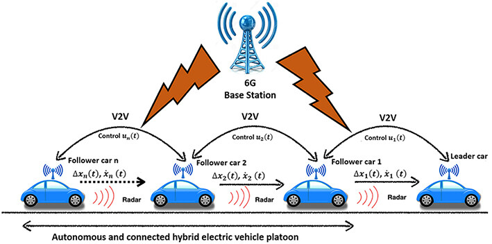
Figure 1. Schematic representation of the CACC system is shown.
The potential impacts of CACC on traffic safety and HEV energy efficiency are a promising field of study because CACC vehicles are expected to penetrate the market more in the near future, and cooperative communication of HEVs with the nearby HEVs using 6G-V2X communication can boast global fuel-saving and traffic safety. Although the aforementioned works contribute to the research in the development of EMSs for HEVs under platooning, there is still a lack of thorough comparative study of the car-following models for fuel efficiency and traffic safety under cooperative driving scenarios. To this end, the following contributions are made: (a) A comparative investigation of IDM, GHR, and OVM microscopic traffic flow models is utilized under connected and cooperative driving scenarios to demonstrate their potential impacts on global energy savings for HEVs; (b) The proposed ECMS is used to further explore the capacity of energy-saving potential of HEVs in a platoon by incorporating the CACC coordinated traffic information in a fuel optimal manner; (c) Extensive simulation studies are carried out under New European Driving Cycle, Worldwide Harmonized Light Vehicle Test Procedure, Highway Fuel Economy Test, and human-in-the-loop drive cycles to clearly demonstrate the advantages of cooperative HEV platooning control methods in terms of speed deviations, battery charge sustainability, and fuel economy.
The rest of the paper is structured as follows. Section 2 presents the control-oriented powertrain model for HEVs along with power flow management. Section 3 introduces the car-following models and Section 4 explains the design of cooperative platoon formation for automated and connected HEVs using car-following models. Extensive simulation studies are demonstrated in Section 5. Lastly, conclusions and future research directions are given in Section 6.
2. ENERGY MANAGEMENT PROBLEM FORMULATION
2.1. Internal Combustion Engine Model
Since the internal combustion engine is a complex system that includes many components, an experimental dataset as a function of engine speed and engine torque is used in this study. The engine speed and torque express the engine fuel consumption ratio by Equations (1), and Equation (2) denotes the engine torque as follows.
where
2.2. Electric Motor Model
The purpose of electric motor (EM) modeling is to obtain the motor power based on motor speed. By ignoring the effect of the dynamic properties of the EM, Equation (3) expresses the efficiency of the motor as a function of the motor speed and motor torque. Then, the required engine power is defined by Equation (4).
where
2.3. Control-Oriented Powertrain Model
Taking advantage of the mixed powertrain configuration (both series and parallel) [42], a power-split HEV model of Toyota Prius is adopted in this study. This HEV powertrain model has been successfully used and commercialized as it has the advantages of the mixed configuration[43, 44]. The power-split HEV model is shown in Figure 2.
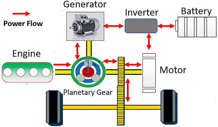
Figure 2. Structure of power-split hybrid electric vehicles [14].
The whole powertrain components of the power-split HEV include one engine, generator/motor (M/G1 and M/G2). The planetary gear set implementation achieves power splitting functionality where the engine is connected to the planet carrier, M/G1 is connected to the sun gear, and a torque coupler is used to combine the ring gear with the M/G2 to power the final drive [45, 46]. Figure 3 shows the structure of the planetary gear system. The kinematic equation of the gear system can be derived as the angular velocities of the sun gear, ring gear, and planet carrier.
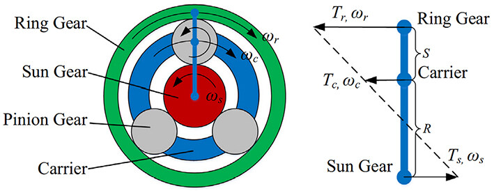
Figure 3. Structure and lever diagram of the planetary gear system equipped in a power-split HEV.
where the radius of the sun gear and the ring gear are denoted by
where the inertias of the generator, engine, and motor are denoted by
where
where empirical data for the engine, generator, and motor are
where
where
Equations (5)–(17) explains the energy management-oriented model used in this paper. The main parameters of the power-split hybrid electric vehicle are given in Table 1.
| Component | Parameter | Value |
| Internal Combustion Engine | Type | Four-cylinder in-line gasoline engine |
| Maximum power | 57 kW @ 4500 RPM | |
| Maximum torque | 110 Nm @ 4500 RPM | |
| Electric motor | Type | AC motor |
| Maximum power | 35 kW @ 1040-5600 RPM | |
| Maximum torque | 30 kW @ 3000-5500 RPM | |
| Battery | Energy capacity | 5 kWh/battery pack |
| Charging capacity | 2.3 Ah/battery unit | |
| Battery cell layout | 110 serial |
2.4. Equivalent consumption minimization
Taking advantage of a real-time energy optimization strategy, ECMS does not require entire driving cycle information in advance, and, by converting electricity consumption to equivalent fuel consumption as well as considering the constraints in engine, motor, generator, and battery, instantaneous equivalent fuel consumption is minimized. To this end, the equivalent factor (EF) is required to convert the electricity consumption into equivalent fuel consumption. The general formulation for the above-mentioned problem is given below.
subject to
where
3. CAR-FOLLOWING MODELS
A car-following model is used to control the driver's behavior, such as maintaining a safe distance and desired reference velocity tracking considering the vehicle ahead in traffic. The following vehicle adjusts its speed according to the preceding vehicle for comfortable driving and safe braking distance [51]. Although the follower's action is usually specified through its acceleration, in some models, the follower's action is defined with the follower's speed [52]. Meanwhile, car-following models use different formulas to describe the follower's behavior. In this work, we introduce three different types of car-following models for the most basic driving behavior to construct reliable models for the development of energy management problems of HEVs under connected driving.
3.1. Intelligent Driver Model
The Intelligent Driver Model (IDM) was developed by Treiber, Hennecke, and Helbing in 2000, which is a type of adaptive cruise control system designed to set the desired longitudinal speed and safety time interval of the driver. It is a type of car-following model that can adjust the driver's behavior according to the changing traffic. To this end, in the IDM, the follower vehicle acceleration varies depending on the distance and speed of the preceding vehicle. In the IDM, the
where
where
where
The desired distance
3.2. Gazis–Herman–Rothery (GHR) Model
The GHR model, also known as the General Motors (GM) model, is developed by Gazis–Herman–Rothery in the 1950s. The GHR model is a stimulus-based car following model [31]. GHR model assumes that the following vehicle responds to arbitrarily small changes in relative speed. GHR model also considers that the follower vehicle responds to the actions of the preceding vehicle, even though the distance to the preceding vehicle is very large, and the follower vehicle's response vanishes as the relative velocity is zero. In the GHR model, the acceleration of the follower vehicle, i.e.,
where
3.3. Optimal Velocity Model
The Optimal Velocity Model (OVM) is a dynamic equation-based car-following model developed by Bando, Hasebe, Nakayama, and Shibata in 1955. According to the OVM, the movement of the vehicle is controlled by an optimal speed. Therefore, in the OVM, the acceleration of the vehicle is calculated based on the difference between the optimal speed and the speed of the vehicle. In the OVM, the acceleration of the
where
where
The values of the above-mentioned models are shown in Table 2[54, 55].
The values of the parameters used in the vehicle following models
| Model | Parameter and values |
| IDM | ( |
| GHR | (c, m, l) = (125, 0.2, 1.6) |
| OVM |
4. CACC PLATOON EXTENSION OF CAR-FOLLOWING MODELS
As an advanced driver assistance system, ACC helps vehicles follow the leading vehicle at a predefined gap by adjusting the vehicle velocity. CACC is an extension of ACC using wireless communication between connected traffic vehicles in a platoon. Connectivity in a CACC system allows vehicles to react more quickly to instantaneous changes than drivers in an ACC system. Furthermore, a CACC system greatly improves safety and mobility in the case of driver distractions and types, and it decreases the negative environmental impacts of emissions. With the help of reliable connectivity between vehicles, CACC enables the execution of appropriate energy management control strategies for HEVs by reducing driver's tasks. To implement classical car-following behavior models under a CACC platoon, we develop a system-level approach to the car-following models that allow adjustment of the vehicle's speed and minimum headway simultaneously with respect to the vehicular state data from multiple vehicles in the CACC platoon. The main underlying idea is that each vehicle in the platoon can react simultaneously to the leader's speed while considering the information of the preceding vehicle [56] in the platoon. For instance, in a platoon of one leader and six follower vehicles, the first following vehicle receives the state information (position, velocity, and acceleration) of the leader in the platoon; likewise, the first follower behaves as a leader vehicle for the vehicle immediately behind and receives the new leader information in real-time. Based on this, the follower vehicles adjust their own state based on the immediately received information of the preceding vehicle in the platoon. As an emerging technology, in the 6G-V2X environment, vehicles can obtain a massive amount of traffic information where CACC vehicles can be coordinated to improve traffic flow efficiency and throughput as well as energy. The closed-loop system of this research is illustrated in Figure 4. In this work, we adopt three commonly used car-following models in the development of a CACC system for HEVs. The proposed scheme can be employed using ordinary differential equations under a platoon of
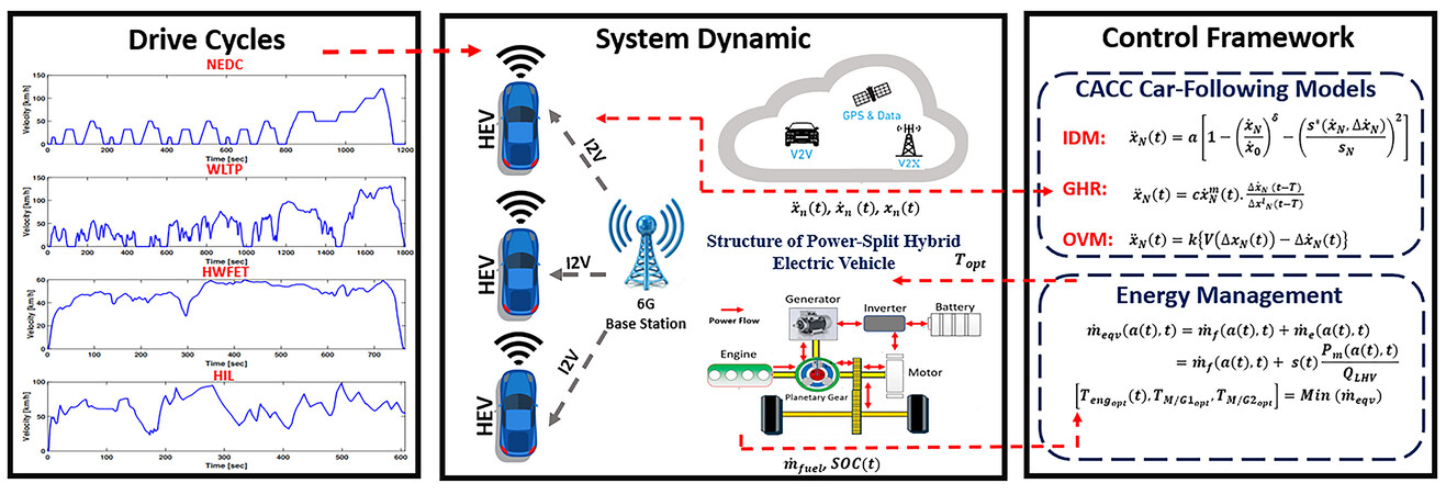
Figure 4. Control hierarchy of the proposed approaches.
4.1. IDM
In the IDM, the follower vehicle acceleration depends on the speed and position of the vehicle in front of it. With the help of the following quadratic ordinary differential equation formulations, the IDM car-following model is converted to a CACC-based model for
where
that is
where
where
4.2. GHR
In the GHR, the acceleration of the follower vehicle depends on the speed and position of the vehicle in front of it. With the help of the following quadratic ordinary differential equation formulations, the OVM car-following model is converted to a CACC-based model for
Then, the system of differential equation of
where
where
4.3. OVM
In the OVM, the acceleration of the follower vehicle depends on the speed and position of the vehicle in front of it. With the help of the following quadratic ordinary differential equation formulations, the OVM car-following model is converted to a CACC-based model for
where
The system of differential equations of
where
5. EXPERIMENT RESULTS
Experiments of a homogeneously connected HEV platoon consisting of one leader and six followers were performed to validate the performance of the energy management algorithms under CACC car-following models to demonstrate the reference velocity trajectory performance and fuel economy advantage. The homogeneous platoon refers to all HEVs having the same powertrain parameters in the platoon. The proposed CACC car-following algorithms were written in MATLAB's embedded function blocks and were run online in Simulink with the ECMS algorithm, forming the CACC-ECMS scheme. The leader vehicle exchanges its state information with the follower vehicles in the connected vehicle platoon via 6G-V2X communication. As for the communication topology in the platoon, vehicles are interconnected via predecessor-following communication topology, meaning that followers receive the state information from their preceding vehicles. It is assumed that the CACC-ECMS scheme works on the 6G-V2X network environment, in which the HEVs are considered to travel on a single-lane road. The 6G base station provides network services to the HEVs where each HEV in the CACC-ECMS scheme communicates with the base station to receive target traffic states such as reference velocities, as shown in Figure 1. To ensure traffic safety and fuel efficiency while cruising in the lane, the HEVs compute control inputs and transmit the inputs by cooperative communication. The HEVs in the CACC-ECMS method employ the ultra-low-latent 6G-V2X communication and periodically broadcast the vehicles' state data, such as relative speeds and the gaps between HEVs.
The proposed CACC-ECMS control strategy is examined under four different types of driving conditions, i.e., NEDC, WLTP, HWFET, and HIL drive cycles. NEDC is a driving cycle that represents the typical use of a car in Europe, consisting of four repeated urban driving cycles and one extra-urban driving cycle. NEDC lasts 1200 s, and the vehicle can accelerate to a maximum speed of 120 km/h. The total distance covered in this driving cycle is 11.01 km. WLTP represents a driving cycle compatible with the world average driving conditions for light vehicles. In WLTP, the driving cycle is 1800 s, and the vehicle can accelerate to a maximum speed of 131.33 km/h. The total distance covered in this driving cycle is 23.25 km. HWFET represents a driving cycle for light vehicles that provide fuel economy on the highway. The HWFET driving cycle lasts 765 s, in which the vehicle accelerates to a maximum speed of 60 km/h. The total distance covered in this driving cycle is 16.45 km. The HIL driving cycle consists of 600 s, in which the driver accelerates to a maximum speed of 98 km/h. The total distance covered in this driving cycle is 11.66 km. The HIL profile is obtained through the setup, as given in Figure 5. The speed profiles of the NEDC, WLTP, HWFET and HIL driving cycles are given in Figure 6. The driving cycles are provided to the leader vehicle via the 6G-V2X channel as the velocity profile in the platoon. Instantaneous velocities of HEVs are shared over 6G-V2V communication, where we examine how the followers react to the speed change of their leader in the platoon from the perspectives of reference velocity following, SOC charge sustainability, and fuel consumption as the ultimate goal. The research ideas of this article are demonstrated in Figure 4.
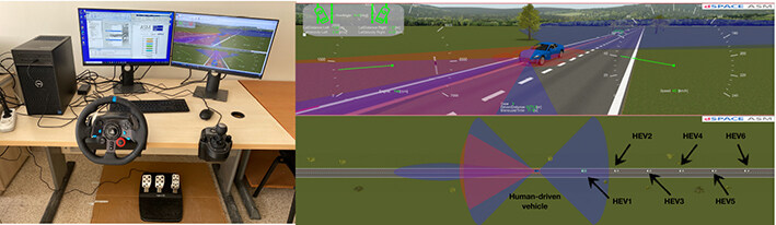
Figure 5. http://lab.tarsus.edu.tr/cars. dSPACE is a high-fidelity driving simulator that offers several block sets for testing and validating vehicle control algorithms. The experiments were performed on a computer equipped with an Intel
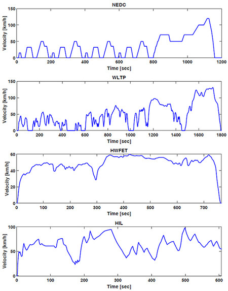
Figure 6. Velocity profile of the driving cycles.
The following part presents the results of four simulation scenarios under NEDC, WLTP, HWFET, and HIL drive cycles so that the driving and energy-saving performances of connected vehicles can be validated in the platoon.
5.1. Driving performance verification results of CACC-ECMS scheme under NEDC, WLTP, HWFET, and HIL driving cycles
In this section, the effectiveness of the CACC-ECMS driving performance, which includes reference speed deviation of the follower vehicles with respect to the preceding vehicles, is assessed. Since the speed trajectory following is an important evaluation index in the platoon, we aim to minimize the deviations of the velocity between vehicles, therefore ensuring string stability. Figures 7–10 show the reference speed trajectory deviations of the vehicles in the platoon under NEDC, WLTP, HWFET, and HIL driving cycles. In Figure 7, we can observe the velocity fluctuations of the follower vehicles with respect to their leader vehicles using three different car-following models. One observation made is that the GHR-based CACC-ECMS model performs better under NEDC cooperative driving cycle than the OVM- and IDM-based CACC-ECMS schemes. However, the GHR- and OVM-based CACC-ECMS methods put more effort than the IDM-based CACC-ECMS method into car-following; thus, HEVs consume more fuel in the platoon, as shown in Table 3. Similarly results are seen in Figures 8 and 9. In Figure 8, the GHR- and OVM-based CACC-ECMS schemes perform better in the car-following mode than that of the IDM-based CACC-ECMS method, as zoomed in the figure. The tradeoff between cooperative driving performance and fuel economy exists under WLTP cycle as well. To show this, the CACC-ECMS scheme results for each car-following model are illustrated under HWFET cycle. In Figure 9, the GHR- and OVM-based CACC-ECMS schemes perform relatively well compared to the IDM-based CACC-ECMS case, where its fuel economy performance is the best in this case as well. The design is also tested in a driving simulator, dSPACE software, which is a high-fidelity driving simulator to test and validate the proposed approach. To this end, a human-in-the-loop driving simulator is an immediate and economical solution to explore the energy-saving potentials of a cooperative hybrid electric vehicle platoon under the presence of a leader vehicle driver style. The simulator is demonstrated in Figure 5. The driver controls the steering wheel, the throttle pedal, and the braking pedal. In the environment, a straight road cooperative driving condition is created, where the human driver controls the leader vehicle and six HEV followers are in the platoon for a driving test. As shown in Figure 10, the GHR- and OVM-based CACC-ECMS schemes perform better in the car-following mode than that of the IDM-based CACC-ECMS method, as zoomed in the same figure. It is seen that driver's speed profile is fluctuating; thus, the follower HEVs cannot effectively track the velocity trajectory of the preceding HEV using the IDM. It is worth noting that the tradeoff between cooperative driving performance and fuel economy exists under this cycle as well.
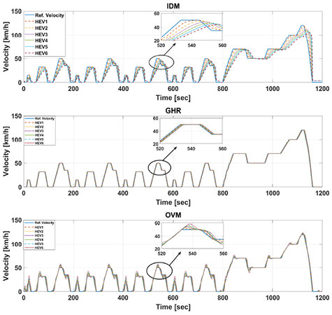
Figure 7. Speed profiles of car following models under NEDC driving cycle.
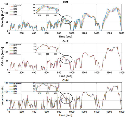
Figure 8. Speed profiles of car following models under WLTP driving cycle.
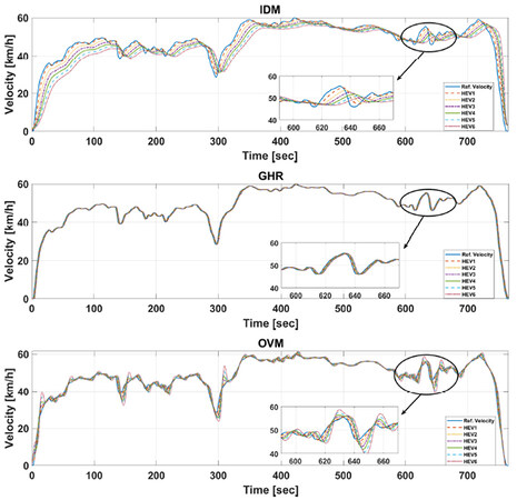
Figure 9. Speed profiles of car following models under HWFET driving cycle.
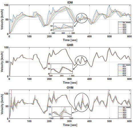
Figure 10. Speed profiles of car following models under HIL driving cycle.
Fuel consumption table of HEVs under different driving cycles
| Drive cycle | Car Following Model | HEV | Fuel consumption (L) | The amount of fuel consumed per 100 km (L/100 km) | Drive cycle | Car Following Model | HEV | Fuel consumption (L) | The amount of fuel consumed per 100 km (L/100 km) | |
| NEDC | IDM | HEV1 | 0.327 | 2.972 | HWFET | IDM | HEV1 | 0.267 | 1.623 | |
| HEV2 | 0.317 | 2.881 | HEV2 | 0.263 | 1.598 | |||||
| HEV3 | 0.308 | 2.799 | HEV3 | 0.259 | 1.574 | |||||
| HEV4 | 0.299 | 2.718 | HEV4 | 0.256 | 1.556 | |||||
| HEV5 | 0.291 | 2.645 | HEV5 | 0.252 | 1.531 | |||||
| HEV6 | 0.283 | 2.572 | HEV6 | 0.249 | 1.513 | |||||
| Platoon | 1.825 | 16.59 | Platoon | 1.547 | 9.403 | |||||
| GHR | HEV1 | 0.332 | 3.018 | GHR | HEV1 | 0.268 | 1.629 | |||
| HEV2 | 0.332 | 3.018 | HEV2 | 0.268 | 1.629 | |||||
| HEV3 | 0.332 | 3.018 | HEV3 | 0.268 | 1.629 | |||||
| HEV4 | 0.331 | 3.009 | HEV4 | 0.267 | 1.623 | |||||
| HEV5 | 0.331 | 3.009 | HEV5 | 0.267 | 1.623 | |||||
| HEV6 | 0.331 | 3.009 | HEV6 | 0.267 | 1.623 | |||||
| Platoon | 1.991 | 18.09 | Platoon | 1.605 | 9.756 | |||||
| OVM | HEV1 | 0.333 | 3.027 | OVM | HEV1 | 0.267 | 1.623 | |||
| HEV2 | 0.334 | 3.036 | HEV2 | 0.268 | 1.629 | |||||
| HEV3 | 0.337 | 3.063 | HEV3 | 0.268 | 1.629 | |||||
| HEV4 | 0.340 | 3.091 | HEV4 | 0.269 | 1.635 | |||||
| HEV5 | 0.346 | 3.145 | HEV5 | 0.270 | 1.641 | |||||
| HEV6 | 0.347 | 3.154 | HEV6 | 0.271 | 1.647 | |||||
| Platoon | 2.039 | 18.53 | Platoon | 1.615 | 9.817 | |||||
| WLTP | IDM | HEV1 | 0.715 | 3.075 | HIL | IDM | HEV1 | 0.289 | 2.711 | |
| HEV2 | 0.694 | 2.984 | HEV2 | 0.279 | 2.617 | |||||
| HEV3 | 0.677 | 2.911 | HEV3 | 0.272 | 2.551 | |||||
| HEV4 | 0.661 | 2.843 | HEV4 | 0.267 | 2.504 | |||||
| HEV5 | 0.647 | 2.782 | HEV5 | 0.261 | 2.448 | |||||
| HEV6 | 0.635 | 2.731 | HEV6 | 0.255 | 2.392 | |||||
| Platoon | 4.030 | 17.33 | Platoon | 1.623 | 15.22 | |||||
| GHR | HEV1 | 0.727 | 3.126 | GHR | HEV1 | 0.306 | 2.869 | |||
| HEV2 | 0.726 | 3.122 | HEV2 | 0.305 | 2.861 | |||||
| HEV3 | 0.726 | 3.122 | HEV3 | 0.304 | 2.851 | |||||
| HEV4 | 0.725 | 3, 117 | HEV4 | 0.304 | 2.851 | |||||
| HEV5 | 0.725 | 3, 117 | HEV5 | 0.303 | 2.842 | |||||
| HEV6 | 0.725 | 3, 117 | HEV6 | 0.302 | 2.833 | |||||
| Platoon | 4.355 | 18.73 | Platoon | 1.825 | 17.11 | |||||
| OVM | HEV1 | 0.732 | 3.148 | OVM | HEV1 | 0.311 | 2.917 | |||
| HEV2 | 0.739 | 3.178 | HEV2 | 0.317 | 2.973 | |||||
| HEV3 | 0.748 | 3.217 | HEV3 | 0.324 | 3.039 | |||||
| HEV4 | 0.756 | 3.251 | HEV4 | 0.332 | 3.114 | |||||
| HEV5 | 0.769 | 3.307 | HEV5 | 0.343 | 3.217 | |||||
| HEV6 | 0.785 | 3.376 | HEV6 | 0.356 | 3.335 | |||||
| Platoon | 4.529 | 19.47 | Platoon | 1.985 | 18.62 |
Some conclusions can be drawn as follows: (i) The tradeoff between reference velocity following of followers versus the fuel consumption of the platoon shows that the driving performance metric is conflicted with the consumed fuel in the platoon; (ii) Even though the GHR-based CACC-ECMS method represents the best driving performance in terms of the reference speed trajectory following, we cannot state its fuel economy is the worst because the fuel economy is also affected by the different model parameters of the proposed scheme.
5.2. Energy saving performance verification results of CACC-ECMS scheme under NEDC, WLTP, HWFET, HIL driving cycles
The effectiveness of the CACC-ECMS scheme is evaluated for energy-saving potential in the platoon in this section. Figures 11–14 show the SOC trajectory deviations of the vehicles in the platoon under NEDC, WLTP, and HWFET driving cycles. The SOC initial value, which is 60%, is to be sustained over the entire driving cycle. Figure 11 shows that the SOC levels with GHR and OVM models are closer to the reference level for each HEV under NEDC cycle in the platoon. We can also observe end-of-cycle SOC values in Table 4. This is indeed a good indicator of the proposed scheme, especially in terms of predictability of its trajectory using GHR and OVM models under NEDC drive cycle, so that the battery works in low resistance. One drawback of this approach is that the fuel economy is deteriorated for the members of the platoon as compared with using IDM under the same drive cycle, as seen in Table 3. The platoon fuel economy per 100 km (L/100 km) is 16.59 L using IDM, while it is 18.09 and 18.53 L using GHR and OVM, respectively. Figure 12 represents SOC findings using the CACC-ECMS scheme under WLPT drive cycle. We can observe that, similar to the NEDC case, the GHR and OVM models exhibit close values to the reference SOC level, while SOC level fluctuates around the reference level using IDM. However, the IDM-based CACC-ECMS scheme presents better fuel-saving, i.e., 17.33 L/100 km, while it is 18.73 and 19.47 L /100 km using GHR and OVM, respectively, in the platoon. Table 3 presents each HEV fuel consumption using different car-following models, subsequently global fuel-savings in the platoon. We can also observe end-of-cycle SOC values using the GHR-based CACC-ECMS scheme in Table 4. SOC trajectories of the proposed CACC-ECMS scheme under HWFET drive cycle are illustrated in Figure 13. Since HWFET cycle is a standard highway, we expect the battery SOC level to be maintained closer to the reference value, as seen in the figure. Even though all car-following models present a similar pattern, only the IDM-based SOC level deviates around the reference level for each HEV in the platoon. Similar to the previous cases, the fuel economy result of the IDM-based CACC-ECMS scheme shows improvements among the HEVs and the platoon relative to the other cases. For this driving cycle, the platoon fuel economy per 100 km (L/100 km) is 9.403 L using IDM, while it is 9.756 and 9.817 L using GHR and OVM, respectively. Lastly, SOC trajectories of the proposed CACC-ECMS scheme under HIL drive cycle are illustrated in Figure 14. The figure shows that the SOC levels deviate around the reference level for each HEV in the platoon only in the OVM case. The fluctuations in the speed profile deteriorate the string stability and energy consumption of HEVs in the platoon. In this aspect, for this driving cycle, the platoon fuel economy per 100 km (L/100 km) is 15.22 L using IDM, while it is 17.11 and 18.62 L using GHR and OVM, respectively.
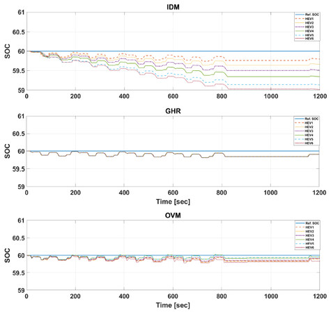
Figure 11. NEDC drive cycle SOC graph.
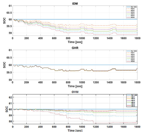
Figure 12. WLTP drive cycle SOC graph.
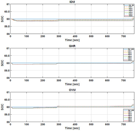
Figure 13. HWFET drive cycle SOC graph.
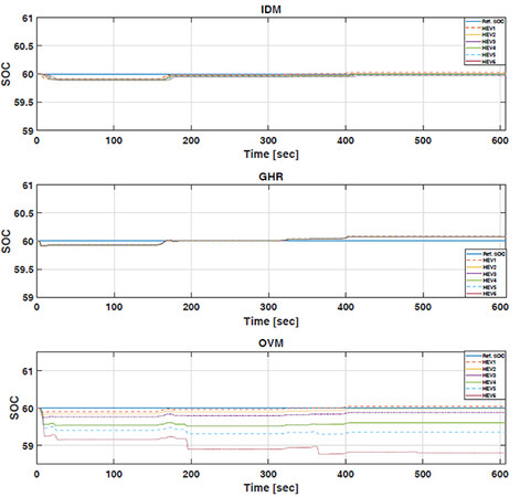
Figure 14. HIL drive cycle SOC graph.
End-of-cycle SOC values of HEVs under different driving cycles
| Drive Cycle | Car Following Model | HEV | SOC(%) | Drive Cycle | Car Following Model | HEV | SOC(%) | |
| NEDC | IDM | HEV1 | 59.81 | HWFET | IDM | HEV1 | 60.08 | |
| HEV2 | 59.68 | HEV2 | 60.05 | |||||
| HEV3 | 59.53 | HEV3 | 60.01 | |||||
| HEV4 | 59.35 | HEV4 | 59.99 | |||||
| HEV5 | 59.14 | HEV5 | 59.95 | |||||
| HEV6 | 59.02 | HEV6 | 59.92 | |||||
| GHR | HEV1 | 59.91 | GHR | HEV1 | 60.10 | |||
| HEV2 | 59.91 | HEV2 | 60.10 | |||||
| HEV3 | 59.91 | HEV3 | 60.10 | |||||
| HEV4 | 59.91 | HEV4 | 60.10 | |||||
| HEV5 | 59.90 | HEV5 | 60.10 | |||||
| HEV6 | 59.90 | HEV6 | 60.09 | |||||
| OVM | HEV1 | 59.89 | OVM | HEV1 | 60.11 | |||
| HEV2 | 59.89 | HEV2 | 60.12 | |||||
| HEV3 | 59.91 | HEV3 | 60.13 | |||||
| HEV4 | 59.95 | HEV4 | 60.13 | |||||
| HEV5 | 59.95 | HEV5 | 60.13 | |||||
| HEV6 | 59.96 | HEV6 | 60.17 | |||||
| WLTP | IDM | HEV1 | 59.67 | HIL | IDM | HEV1 | 60.03 | |
| HEV2 | 59.49 | HEV2 | 60.01 | |||||
| HEV3 | 59.35 | HEV3 | 60.00 | |||||
| HEV4 | 59.20 | HEV4 | 59.99 | |||||
| HEV5 | 59.05 | HEV5 | 59.98 | |||||
| HEV6 | 58.91 | HEV6 | 59.97 | |||||
| GHR | HEV1 | 59.77 | GHR | HEV1 | 60.09 | |||
| HEV2 | 59.76 | HEV2 | 60.08 | |||||
| HEV3 | 59.75 | HEV3 | 60.08 | |||||
| HEV4 | 59.75 | HEV4 | 60.08 | |||||
| HEV5 | 59.74 | HEV5 | 60.08 | |||||
| HEV6 | 59.74 | HEV6 | 60.07 | |||||
| OVM | HEV1 | 59.86 | OVM | HEV1 | 60.04 | |||
| HEV2 | 59.85 | HEV2 | 59.97 | |||||
| HEV3 | 59.79 | HEV3 | 59.88 | |||||
| HEV4 | 59.49 | HEV4 | 59.60 | |||||
| HEV5 | 58.87 | HEV5 | 59.35 | |||||
| HEV6 | 57.84 | HEV6 | 58.80 |
One main conclusion can be drawn for all cases: the IDM-based CACC-ECMS scheme provides the best fuel economy, while there are tradeoffs for the SOC reference trajectory following performance under various drive cycles. The GHR-based CACC-ECMS scheme performs relatively better than the OVM-based scheme for energy-saving, and both methods present a similar SOC trajectory following performance under NEDC and HWFET drive cycles.
6. CONCLUSION
This work proposes a hybrid electric vehicle (HEV) platoon control using car-following model-based cooperative adaptive cruise control (CACC). Utilizing sixth-generation vehicle-to-everything (6G-V2X) communications network service for connected and automated HEV platoon, HEVs are capable of communicating with the base station to receive target traffic states such as reference velocities and positions. Using the obtained traffic data, an equivalent consumption minimization strategy (ECMS) is used for power flow management, where the velocities of leader vehicles are used for cooperative driving as well as energy-saving. With the help of the predecessor-following communication topology in the platoon, the proposed CACC-ECMS framework fully explores the advantage of fuel consumption reduction while ensuring string stability. Experiments under different drive cycles result in the following conclusions:
● The GHR- and OVM-based CACC-ECMS schemes present better car-following performance than that of the IDM-based CACC-ECMS scheme at the cost of fuel consumption.
● The SOC reference trajectory following performance of the GHR- and OVM-based CACC-ECMS schemes is better in terms of target deviation over the entire drive cycles than that of the IDM-based CACC-ECMS approach.
● In the platoon, the IDM-based CACC-ECMS consumes fuel at 16.59 L/100 km under NEDC, 17.33 L/100 km under WLTP, 9.403 L/100 km under HWFET, and 15.22 L/100 km under HIL. The GHR-based CACC-ECMS consumes fuel at 18.09 L/100 km under NEDC, 18.73 L/100 km under WLTP, 9.756 L/100 km under HWFET, and 17.11 L/100 km under HIL. The OVM-based CACC-ECMS consumes fuel at 18.53 L/100 km under NEDC, 19.47 L/100 km under WLTP, 9.817 L/100 km under HWFET, and 18.62 L/100 km under HIL.
● The IDM-based CACC-ECMS is an energy-efficient strategy that saves: (i) 8.29% fuel compared to the GHR-based CACC-ECMS and 10.47% compared to the OVM-based CACC-ECMS under NEDC; (ii) 7.47% fuel compared to the GHR-based CACC-ECMS and 11% compared to the OVM-based CACC-ECMS under WLTP; (iii) 3.62% fuel compared to the GHR-based CACC-ECMS and 4.22% compared to the OVM-based CACC-ECMS under HWFET; and (iv) 11.05% fuel compared to the GHR-based CACC-ECMS and 18.26% compared to the OVM-based CACC-ECMS under HIL.
Future work will be directed toward the influence of the interaction of vehicles on energy-saving potentials. The negative impacts of communication outage on energy-saving deterioration will also be investigated.
Symbols and abbreviations in the article are given in Table 5.
Symbols and abbreviations
| Symbols | |||
| $$ {\dot{m}}_{eqv}$$ | Equivalent fuel consumption | $$C$$ | Carrier gear |
| $$ {\dot{m}}_{fuel}$$ | Engine fuel consumption | $$R$$ | Ring gear |
| $$ {\dot{x}}_0$$ | Desired velocity of the vehicle $n$th | $$S$$ | Sun gear |
| $$ {\ddot{x}}_n$$ | Acceleration of the $n$th vehicle $n$th | $$T$$ | Safe time headway |
| $$ {\dot{x}}_n $$ | Velocity of the $n$th vehicle | $$T_m$$ | Electric motor torque |
| $$ \mathrm{\Psi}_{eng}$$ | Engine empirical data | $$b$$ | Maximum deceleration |
| $$ \mathrm{\Psi}_{M/G1}$$ | Generator empirical data | $$g$$ | Gravitational acceleration |
| $$ \mathrm{\Psi}_{M/G2}$$ | Motor empirical data | $$m$$ | Vehicle mass |
| $$C_{d}$$ | Rolling resistance coefficient | $$n_m$$ | Electric motor speed |
| $$I_{batt}$$ | Battery current | $$s$$ | Equivalent factor |
| $$I_{M/G1}$$ | Generator inertia | $$ \alpha$$ | Engine throttle |
| $$I_{M/G2}$$ | Motor inertia | $$ \delta$$ | Exponent for vehicle's acceleration |
| $$I_{eng}$$ | Engine inertia | $$ \theta$$ | Road grade |
| $$g_{f}$$ | Gear ratio of final drive | Abbrevations | |
| $$P_{batt}$$ | Battery power | ACC | Adaptive cruise control |
| $$P_m$$ | Electric motor power | CACC | Cooperative adaptive cruise control |
| $$Q_{max}$$ | Capacity of battery | CAV | Connected and automated vehicle |
| $$R_{batt}$$ | Internal resistance | ECMS | Equivalent consumption minimization strategy |
| $$R_{wheel}$$ | Radius of wheel | EF | Equivalent factor |
| $$T_{axle}$$ | Axle torque | EM | Electric motor |
| $$T_{brake}$$ | Brake torque | EMS | Energy management system |
| $$T_{e}$$ | Engine torque | GHR | Gazis--Herman--Rothery model |
| $$T_{e max}$$ | Engine maximum torque | HEV | Hybrid electric vehicle |
| $$V_{oc}$$ | Open circuit voltage | HWFET | Highway fuel economy test |
| $$l_n$$ | Vehicle length | ICE | Internal combustion engine |
| $$n_{e}$$ | Engine speed | IDM | Intelligent driver model |
| $$s_0$$ | Minimum space | ITS | Intelligent transportation system |
| $$ \eta_{inv}$$ | Inverter efficiency | MPC | Model predictive control |
| $$ \eta_{m}$$ | Electric motor efficiency | NEDC | New European driving cycle |
| $$ \omega_C$$ | Carrier gear angular velocity | OVM | Optimal velocity model |
| $$ \omega_{eng}$$ | Engine angular speed | PMP | Pontryagin's minimum principle |
| $$ \omega_{ M/G1}$$ | $$M/G1$$ angular speed | SOC | State of charge |
| $$ \omega_{ M/G2}$$ | $$M/G2$$ angular speed | V2I | Vehicle-to-infrastructure |
| $$ \omega_R$$ | Ring gear angular velocity | V2V | Vehicle-to-vehicle |
| $$ \omega_S$$ | Sun gear angular velocity | V2X | Vehicle-to-everything |
| $$ \Delta \dot{x}_n$$ | Distance between vehicles | WLTP | Worldwide harmonized light vehicles test procedure |
| $$N$$ | number of vehicles in platoon | 6G | sixth generation |
| $$F$$ | Internal force on pinion gears | 6G-V2X | sixth-generation vehicle-to-everything |
DECLARATIONS
Acknowledgments
The authors would like to thank the anonymous reviewers for their valuable comments.
Authors' contributions
Made substantial contributions to conception, manuscript preparation, experimental studies, and manuscript editing/revision: Yazar O, Coskun S
Made substantial contributions to reviewing/editing and technical notes: Zhang F, Li L
Availability of data and materials
Not applicable.
Financial support and sponsorship
This study is supported by the Scientific and Technological Research Council of Turkey with Project No. 121E260 under the grant name CAREER.
Conflicts of interest
All authors declared that there are no conflicts of interest.
Ethical approval and consent to participate
Not applicable.
Consent for publication
Not applicable.
Copyright
© The Author(s) 2022.
REFERENCES
1. Saiteja P, Ashok B. Critical review on structural architecture, energy control strategies and development process towards optimal energy management in hybrid vehicles. Energy Reviews 2022;157:112038.
2. Zhang F, Hu X, Langari R, Cao D. Energy management strategies of connected hevs and phevs: Recent progress and outlook. Progress in Energy and Combustion Science 2019;73:235-56.
3. Li L, Coskun S, Wang J, Fan Y, Zhang F, Langari R. Velocity prediction based on vehicle lateral risk assessment and traffic flow: A brief review and application examples. Energies 2021;14:3431.
4. Yadlapalli RT, Kotapati A, Kandipati R, Koritala CS. A review on energy efficient technologies for electric vehicle applications. J Energy Storage 2022;50:104212.
5. Ruan S, Ma Y, Yang N, Xiang C, Li X. Real-time energy-saving control for HEVs in car-following scenario with a double explicit MPC approach. Energy 2022;247:123265.
6. Hu X, Wang H, Tang X. Cyber-physical control for energy-saving vehicle following with connectivity. IEEE Trans Ind Electron 2017;64:8578-87.
7. Kannan Chidambaram, Bragadeshwaran Ashok, Rajasekar Vignesh, Chirag Deepak, Rathan Ramesh, Tharun MV Narendhra, Kaisan Muhammad Usman, and Chellapan Kavitha. Critical analysis on the implementation barriers and consumer perception toward future electric mobility. Proceedings of the Institution of Mechanical Engineers, Part D: Journal of Automobile Engineering, page 09544070221080349, 2022.
8. Liu Z, Lee H, Khyam M, et al. 6g for vehicle-to-everything (v2x) communications: Enabling technologies, challenges, and opportunities. arXiv preprint arXiv: 2012.07753, 2020.
9. Prathiba SB, Raja G, Kumar N. Intelligent cooperative collision avoidance at overtaking and lane changing maneuver in 6g-v2x communications. IEEE Trans Veh Technol 2022;71:112-22.
10. Yang C, Zha M, Wang W, Liu K, Xiang C. Efficient energy management strategy for hybrid electric vehicles/plug-in hybrid electric vehicles: review and recent advances under intelligent transportation system. IET Intelligent Transport Systems 2020;14:702-11.
11. He H, Wang Y, Han R, Han M, Bai Y, Liu Q. An improved mpc-based energy management strategy for hybrid vehicles using v2v and v2i communications. Energy 2021;225:120273.
12. Zhao Z, Tang P, Li H. Generation, screening, and optimization of powertrain configurations for power-split hybrid electric vehicle: A comprehensive overview. IEEE Trans Transp Electrific 2022;8:325-44.
13. Kannan C, Vignesh R, Karthick C, Ashok B. Critical review towards thermal management systems of lithium-ion batteries in electric vehicle with its electronic control unit and assessment tools. Proceedings of the Institution of Mechanical Engineers, Part D: Journal of Automobile Engineering 2021;235: 1783-807.
14. Zhang F, Wang L, Coskun S, Pang H, Cui Y, Xi J. Energy management strategies for hybrid electric vehicles: Review, classification, comparison, and outlook. Energies 2020;13:3352.
15. Vignesh R, Ashok B. Deep neural network model-based global calibration scheme for split injection control map to enhance the characteristics of biofuel powered engine. Energy Conversion and Management 2021;249:114875.
16. Omanovic A, Zsiga N, Soltic P, Onder C. Optimal degree of hybridization for spark-ignited engines with optional variable valve timings. Energies 2021;14:8151.
17. Onori S, Serrao L, Rizzoni G. Hybrid electric vehicles: Energy management strategies. 2016.
18. Liu T, Tan W, Tang X, Zhang J, Xing Y, Cao D. Driving conditions-driven energy management strategies for hybrid electric vehicles: A review. Renewable and Sustainable Energy Reviews 2021;151:111521.
19. Paganelli G. Design and control of a parallel hybrid car with electric and thermal powertrain. M. Sc 1999.
20. Shi D, Liu S, Cai Y, Wang S, Li H, Chen L. Pontryagin's minimum principle based fuzzy adaptive energy management for hybrid electric vehicle using real-time traffic information. Applied Energy 2021;286:116467.
21. Zhang F, Xiao L, Coskun S, et al. Comparative study of energy management in parallel hybrid electric vehicles considering battery ageing. Energy 2022:123219.
22. Zhang F, Xi J, Langari R. Real-time energy management strategy based on velocity forecasts using v2v and v2i communications. IEEE Trans Intell Transport Syst 2017;18:416-30.
23. Deshpande SR, Jung D, Bauer L, Canova M. Integrated approximate dynamic programming and equivalent consumption minimization strategy for eco-driving in a connected and automated vehicle. IEEE Trans Veh Technol 2021;70:11204-15.
24. Wang W, Guo X, Yang C, et al. A multi-objective optimization energy management strategy for power split hev based on velocity prediction. Energy 2022;238:121714.
25. Chen Z, Liu Y, Ye M, Zhang Y, Chen Z, Li G. A survey on key techniques and development perspectives of equivalent consumption minimisation strategy for hybrid electric vehicles. Renewable and Sustainable Energy Reviews 2021;151:111607.
26. Guanetti J, Kim Y, Borrelli F. Control of connected and automated vehicles: state of the art and future challenges. Annual Reviews in Control 2018;45:18-40.
27. Homchaudhuri B, Lin R, Pisu P. Hierarchical control strategies for energy management of connected hybrid electric vehicles in urban roads. Transportation Research Part C: Emerging Technologies 2016;62:70-86.
28. Pipes LA. An operational analysis of traffic dynamics. Journal of Applied Physics 1953;24:274-81.
29. Chandler RE, Herman R, Montroll EW. Traffic dynamics: studies in car following. Operations Research 1958;6:165-84.
30. Treiber M, Hennecke A, Helbing D. Congested traffic states in empirical observations and microscopic simulations. Phys Rev E Stat Phys Plasmas Fluids Relat Interdiscip Topics 2000;62:1805-24.
31. Gazis DC, Herman R, Rothery RW. Nonlinear follow-the-leader models of traffic flow. Operations Research 1961;9:545-67.
32. Bando M, Hasebe K, Nakayama A, Shibata A, Sugiyama Y. Dynamical model of traffic congestion and numerical simulation. Phys Rev E Stat Phys Plasmas Fluids Relat Interdiscip Topics 1995;51:1035-42.
33. Ioannou P, Chien C. Autonomous intelligent cruise control. IEEE Trans Veh Technol 1993;42:657-72.
34. Fellendorf M, Vortisch P. Microscopic traffic flow simulator vissim. In: Barceló J, editor. Fundamentals of Traffic Simulation. New York: Springer; 2010. pp. 63-93.
35. Li G, Gorges D. Ecological adaptive cruise control and energy management strategy for hybrid electric vehicles based on heuristic dynamic programming. IEEE Trans Intell Transport Syst 2019;20:3526-35.
36. Vajedi M, Azad NL. Ecological adaptive cruise controller for plug-in hybrid electric vehicles using nonlinear model predictive control. IEEE Trans Intell Transport Syst 2016;17:113-22.
37. Jia Y, Jibrin R, Gorges D. Energy-optimal adaptive cruise control for electric vehicles based on linear and nonlinear model predictive control. IEEE Trans Veh Technol 2020;69:14173-87.
38. Ma G, Ghasemi M, Song X. Integrated powertrain energy management and vehicle coordination for multiple connected hybrid electric vehicles. IEEE Trans Veh Technol 2018;67:2893-9.
39. Li J, Zhou Q, He Y, Williams H, Xu H, Lu G. Distributed cooperative energy management system of connected hybrid electric vehicles with personalized non-stationary inference. IEEE Trans Transp Electrific 2022;8:2996-3007.
40. Ma F, Yang Y, Wang J, et al. Predictive energy-saving optimization based on nonlinear model predictive control for cooperative connected vehicles platoon with v2v communication. Energy 2019;189:116120.
41. Xu L, Zhuang W, Yin G, Bian C. Energy-oriented cruising strategy design of vehicle platoon considering communication delay and disturbance. Transportation Research Part C: Emerging Technologies 2019;107:34-53.
42. Syed FU, Kuang ML, Czubay J, Ying H. Derivation and experimental validation of a power-split hybrid electric vehicle model. IEEE Trans Veh Technol 2006;55:1731-47.
43. Liu J, Peng H. Modeling and control of a power-split hybrid vehicle. IEEE Trans Contr Syst Technol 2008;16:1242-51.
44. Yang Y, Hu X, Pei H, Peng Z. Comparison of power-split and parallel hybrid powertrain architectures with a single electric machine: Dynamic programming approach. Applied Energy 2016;168:683-90.
45. Sun C, Hu X, Moura SJ, Sun F. Velocity predictors for predictive energy management in hybrid electric vehicles. IEEE Trans Contr Syst Technol 2015;23:1197-204.
46. Sun C, Sun F, He H. Investigating adaptive-ecms with velocity forecast ability for hybrid electric vehicles. Applied Energy 2017;185:1644-53.
47. Hu X, Li S, Peng H. A comparative study of equivalent circuit models for li-ion batteries. Journal of Power Sources 2012;198:359-67.
48. Moura SJ, Chaturvedi NA, Krstić M. Adaptive partial differential equation observer for battery state-of-charge/state-of-health estimation via an electrochemical model. Journal of Dynamic Systems, Measurement, and Control 2014;136:011015.
49. Muta K, Yamazaki M, Tokieda J. Development of new-generation hybrid system ths ii-drastic improvement of power performance and fuel economy. Technical report, 2004.
50. Rousseau A, Kwon J, Sharer P, Pagerit S, Duoba M. Integrating data, performing quality assurance, and validating the vehicle model for the 2004 prius using psat. Technical report, SAE Technical Paper, 2006.
51. Treiber M, Kesting A. Traffic flow dynamics. Traffic Flow Dynamics: Data, Models and Simulation, Springer-Verlag Berlin Heidelberg 2013; doi: 10.1007/978-3-642-32460-4.
52. Gipps P. A behavioural car-following model for computer simulation. Transportation Research Part B: Methodological 1981;15:105-11.
53. Brackstone M, Mcdonald M. Car-following: a historical review. Transportation Research Part F: Traffic Psychology and Behaviour 1999;2:181-96.
54. Jiang R, Wu Q, Zhu Z. Full velocity difference model for a car-following theory. Phys Rev E Stat Nonlin Soft Matter Phys 2001;64:017101.
55. Treiterer J, Myers J. The hysteresis phenomenon in traffic flow. Transportation and traffic theory, 6: 13-38 1974;6:13-38.
Cite This Article
Export citation file: BibTeX | RIS
OAE Style
Yazar O, Coskun S, Zhang F, Li L. A comparative study of energy management systems under connected driving: cooperative car-following case. Complex Eng Syst 2022;2:7. http://dx.doi.org/10.20517/ces.2022.06
AMA Style
Yazar O, Coskun S, Zhang F, Li L. A comparative study of energy management systems under connected driving: cooperative car-following case. Complex Engineering Systems. 2022; 2(2): 7. http://dx.doi.org/10.20517/ces.2022.06
Chicago/Turabian Style
Yazar, Ozan, Serdar Coskun, Fengqi Zhang, Lin Li. 2022. "A comparative study of energy management systems under connected driving: cooperative car-following case" Complex Engineering Systems. 2, no.2: 7. http://dx.doi.org/10.20517/ces.2022.06
ACS Style
Yazar, O.; Coskun S.; Zhang F.; Li L. A comparative study of energy management systems under connected driving: cooperative car-following case. Complex. Eng. Syst. 2022, 2, 7. http://dx.doi.org/10.20517/ces.2022.06
About This Article
Copyright

Data & Comments
Data


 Cite This Article 43 clicks

 Like This Article 31
likes
Like This Article 31
likes


Comments
Comments must be written in English. Spam, offensive content, impersonation, and private information will not be permitted. If any comment is reported and identified as inappropriate content by OAE staff, the comment will be removed without notice. If you have any queries or need any help, please contact us at support@oaepublish.com.