
Explainable fuzzy cluster-based regression algorithm with gradient descent learning


Abstract
We propose an algorithm for n-dimensional regression problems with continuous variables. Its main property is explainability, which we identify as the ability to understand the algorithm's decisions from a human perspective. This has been achieved thanks to the simplicity of the architecture, the lack of hidden layers (as opposed to deep neural networks used for this same task), and the linguistic nature of its fuzzy inference system. First, the algorithm divides the joint input-output space into clusters that are subsequently approximated using linear functions. Then, we fit a Cauchy membership function to each cluster, therefore identifying them as fuzzy sets. The prediction of each linear regression is merged using a Takagi-Sugeno-Kang approach to generate the prediction of the model. Finally, the parameters of the algorithm (those from the linear functions and Cauchy membership functions) are fine-tuned using gradient descent optimization. In order to validate this algorithm, we considered three different scenarios: The first two are simple one-input and two-input problems with artificial data, which allow visual inspection of the results. In the third scenario, we use real data for the prediction of the power generated by a combined cycle power plant. The results obtained in this last problem (3.513 RMSE and 2.649 MAE) outperform the state of the art (3.787 RMSE and 2.818 MAE).
Keywords
1. INTRODUCTION
Over the last few years, artificial ntelligence (AI) and Machine Learning (ML) have become ubiquitous in human society. Riding primarily on the empirical success of the deep neural network (DNN), AI and ML have expanded to sectors where safety and accountability must be guaranteed (e.g., medicine and national security) with an increasing emphasis on data privacy and protection. Decisions derived from AI-powered systems in such sectors directly affect people's lives, motivating a need for transparency: explainability and interpretability. Models should make sense to the human observer, and decisions must be justified and legitimate, with detailed explanations that promote trust. Human observers should understand how these decisions are made (the actions or procedures taken by the model) and why they work when they do (or fail when they don't).
The excellent performance of DNNs, however, relies on opaque abstractions in the (often hundreds) of hidden layers and millions of parameters that obscure their decision-making process, leading to the development of black box models which lack a clear understanding of how the model works. This performance – transparency trade-off was historically acceptable since AI-powered systems were deployed primarily for scientific and limited commercial work. The widespread expansion of AI and DNNs outside of academia thus motivates the need for modified machine learning techniques that learn explainable features while maintaining performance, as well as more interpretable, structured causal models.
Measuring explainability is an additional concern. Montavon et al.[1], Vedaldi et al.[2], and Letham et al.[3] are summaries of current techniques used by DNNs. There are seven major ways to achieve interpretability in a model:
The previous mechanisms could be understood as a top-down addition of mathematical tools to increase the interpretability. A less explored approach is the bottom-up redefinition of model architectures such that the algorithms are inherently transparent. In fact, most of the methods that seek to provide the desired transparency in neural networks elaborate on top of the fundamentals and rarely provide a novel algorithmic architecture. For example, Yang et al.[26] introduced an enhanced explainable neural network (ExNN) that decomposes a complex relationship into additive components, where the explainability is obtained by the addition of orthogonality constraints and the sparsity of the generated subnetworks. Similarly, Tran et al.[27] used variational autoencoders to generate interpretable features, and Wolf et al.[28] suggested the visualization of intermediate models to improve the trustworthiness of the system. While these techniques provide more clarity on the decision-making process, they are not easy to generalize and, in fact, are less explainable than a decision tree or a linear regression.
Additionally, minor changes to a DNN's input can negatively impact performance, causing misclassifications or false predictions, leading to the use of fragile models easily fooled by noise. The expansion of AI to mission critical fields thus also motivates the need for robust solutions resilient to noise. Al-Mahasneh et al.[29] introduced a novel evolutionary algorithm that leverages competitive learning strategies to obtain the most optimal network that can handle noisy data. Autoencoders have been very successfully employed for denoising tasks, especially in medical procession [30], and speech enhancement [31]. Nevertheless, all the aforementioned methods hinge on the use of uncorrupted data points in the learning process. Both the noisy and clean instances are shown to the system until it learns to identify noisy patterns and develops its noise suppression strategy – information that is unavailable in most real-world applications. "Truth" often refers to the output values in the data, which in fact, may have a certain percentage of noise from the data acquisition process. Thus, the ground truth remains unknown.
This paper proposes a novel noise-resilient, explainable learning algorithm for
Section II is a description of the algorithm's phases and the corresponding mathematical formulation. Section III describes the data sets used for empirical evaluation, including both synthetic and real-world data. Section IV discusses our empirical results. Section V concludes this paper and offers ideas for future work.
2. PROPOSED ALGORITHM
First, a clustering algorithm divides the joint input-output space into
Then, in each cluster, the dependence of the output
For a generic vector
where
The output of the model is generated by merging the linear functions of the clusters through a Takagi-Sugeno-Kang approach,
where
where
Once the parameters of both the membership functions and the linear functions have been initialized, the model is trained using GD learning. We define the loss function for the data vector as
and the loss over the whole the training set X as
where the factor
The matrix expression of the formulation for the update of the different parameters is
where
and
Equation (7) has been developed minimizing (6), as shown in the Appendix C.
For the update of the parameters, one can think of two different approaches, synchronously and asynchronously. The synchronous approach requires visiting all the observations of the training sample before training the parameters. Thus, in this configuration, there is only one update performed at the end of each epoch. In the asynchronous version, we update the parameters of every cluster after studying an instance of the sample. In this case, we would have as many updates as observations per epoch. The latter requires a higher computational cost, but the evolution of the parameters is more stable and smooth than the synchronous approach. In the results section of this paper, we considered the asynchronous update. These two optimization versions can be visualized in Figure 1.
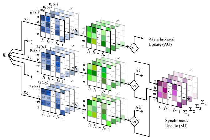
Figure 1. Synchronous and asynchronous approaches for the update of the system's parameters. Each observation of the dataset has a different set of matrices that together constitute the gradient of the loss function (transparent matrices of the back refer to different clusters). The entries of the blue matrices represent the derivatives with respect to the different parameters of the system; the rows determine the type of the parameter,
3. RESULTS
We tested this algorithm in three different problems; 1 input 1 output, 2 inputs 1 output, and 4 inputs 1 output. In the first two cases, we created the data artificially, and in the third application, we used real data obtained from the University of California Irvine (UCI) Machine Learning repository [46]. In this section, we provide a brief revision of the lessons learned from the first two, which were covered in Viaña et al.[47,48], and a detailed explanation of the results obtained in the last scenario.
3.1. Single-input problem
We studied 20 different functions. In order to measure the noise resilience of the method, we injected random noise in the output variable of the training dataset (from a uniform distribution), but the testing data had no noise (the algorithm was never exposed to the ground truth). In each case, we used a ranging number of clusters to evaluate the differences in the approximations obtained. As a benchmark, we utilized a selection of neural networks of one-hidden layer with varying numbers of hidden neurons. The proposed algorithm obtained significantly better results than all the neural network configurations studied [47]. In Figures 2-3, we show the results obtained with both approaches for the function
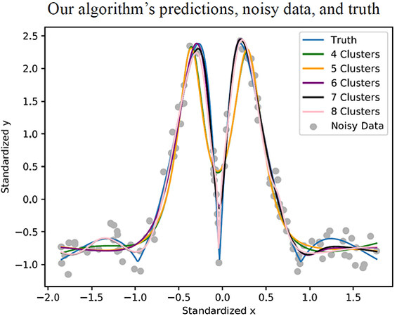
Figure 2. Single input function approximation with the algorithm presented in this paper considering 4, 5, 6, 7 and 8 clusters. The noisy data and the ground truth is also visible. All the systems were trained till the achievement of convergence in the training error.
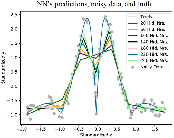
Figure 3. Single input function approximation benchmark with neural networks of architectures ranging from 20 to 260 hidden neurons in steps of 40. The noisy data and the ground truth are also visible. All the systems were trained till the achievement of convergence in the training error.
For the training data, we considered the same 100 noisy observations for both approaches. All the systems were trained using a learning rate of 0.01, and the learning stopped when the loss converged. In all the cases studied, our algorithm converged in 1, 000 epochs, whereas the neural networks required 10, 000.
3.2. Double-input problem
The purpose of this second problem was to prove the applicability of the algorithm to
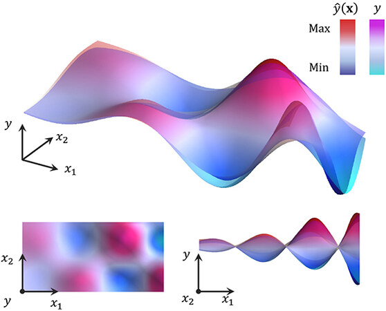
Figure 4. Double input function approximation with the algorithm presented in this paper considering 7 clusters. Both the ground truth and the approximation are visible. Three views are displayed for clarity. The system was trained till we achieved convergence in the training error.
3.3. Four-input problem
In order to prove the applicability of the algorithm with real multidimensional problems, we considered the regression data of a combined cycle power plant (CCPP) [49] from the UCI machine learning repository. A CCPP consists of two types of turbines that generate electricity (gas and steam turbines). Gas turbines take the air and natural gas fuel inlets for the production of electricity at the cost of generating an outlet of exhaust gases at a high temperature. The heat of these gases is recycled with a secondary circuit of water that is evaporated for further extraction of energy in the water turbine. Figure 5 shows the schematic layout of a typical CCPP system, simplified for clarity purposes.
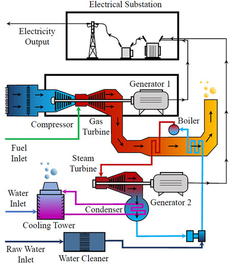
Figure 5. Schematic representation of the Combined Cycle Power Plant layout.
The popularity of such power plants has increased over the last years, particularly in areas with natural gas resources [50]. The CCPP considered for this study has a nominal generating capacity of 480 MW, two 160 MW ABB 13E2 Gas Turbines, two dual pressure Heat Recovery Steam Generators, and one 160 MW ABB Steam Turbine.
The task chosen focuses on the prediction of the electric power produced by the plant when it operates at full load. The ambient temperature, atmospheric pressure, and relative humidity have an impact on the efficiency of the gas turbine, and so does the exhaust steam pressure affect the steam turbine performance. These four variables are considered inputs of the problem, and the power output of the plant, the value we want to predict, is the target. All the observations in the data correspond to the average hourly measurements of the sensors installed in the plant. Table 1 contains some basic statistics of these measures for the dataset selected.
Variables of the Combined Cycle Power Plant problem (publicly available dataset) [49]
| Variable | Min | Max | Mean |
| Ambient Temperature | 1.8℃ | 37.1℃ | 19.6℃ |
| Atmospheric Pressure | 99289 Pa | 103330 Pa | 101326 Pa |
| Relative Humidity | 25.5% | 100% | 73.3% |
| Exhaust Steam Pressure | 3381 Pa | 10874 Pa | 7241 Pa |
| Full Load Power Output | 420.26 MW | 495.76 MW | 454.37 MW |
The dataset consists of 10, 000 observations. We considered 1, 600 randomly chosen instances for training and 800 for testing (0.8 split). We chose a model of 6 clusters, and we trained for 4, 000 epochs with a 0.0001 learning rate (for all the parameters). In order to avoid overtraining, we selected a random sample of 960 training instances randomly chosen from the training set in every epoch (samples of 60% from the training points). We used the root mean squared error (RMSE) and the mean absolute error (MAE) as figures of merit to evaluate the performance of our algorithm. Once the learning process finished, the final RMSE and MAE values of the training set were 3.200 and 2.450, respectively. Similarly, the RMSE and MAE values obtained for the testing set were 3.513 and 2.649. Figures 6-7 show the evolution of the RMSE and MAE over the epochs of the training process while using the GD optimization in our algorithm.
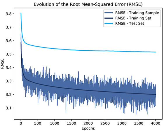
Figure 6. Evolution over epochs of the Root Mean Squared Error's for the training sample, the entire training set, and the test set for the CCPP problem.
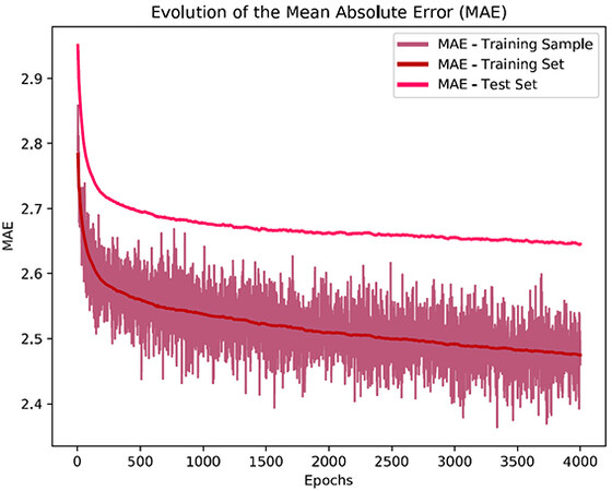
Figure 7. Evolution over epochs of the Mean Absolute Error for the training sample, the entire training set, and the test set for the CCPP problem.
In Tufekci [50], a variety of different methods were studied for this particular CCPP problem. We provide a sum up of the RMSE values obtained in all those approaches together with our results in Table 2.
Comparison of test set RMSE for the different regression algorithms
| Category | Regression Algorithm | Acronym | Reference | RMSE |
| Functions | This Paper's Algorithm | - | - | 3.513 |
| Simple Linear Regression | SLR | [51] | 5.426 | |
| Linear Regression | LR | [52] | 4.561 | |
| Least Median Square | LMS | [53] | 4.572 | |
| Multilayer Perceptron | MLP | [54] | 5.399 | |
| Radial Basis Function NN | RBF | [55] | 8.487 | |
| Pace Regression | PR | [51] | 4.561 | |
| Support Vector Poly Kernel | SVR | [55] | 4.563 | |
| Lazy-learning | IBk Linear NN Search | IBk | [56] | 4.656 |
| KStar | K* | [57] | 3.861 | |
| Locally Weighted Learning | LWL | [56] | 8.221 | |
| Meta-learning | Additive Regression | AR | [58] | 5.556 |
| Bagging REP Tree | BREP | [59] | 3.787 | |
| Rule-based | Model Trees Rules | M5R | [51] | 4.128 |
| Tree-based | Model Trees Regression | M5P | [60] | 4.087 |
| REP Trees | REP | [61] | 4.211 |
Table 3 shows the figures of merit for the top four methods studied by Tufekci [50] and the proposed algorithm.
Sorted list of the best regression algorithms using the test set performances
| Category | Regression Algorithm | Performance | |
| RMSE | MAE | ||
| Functions | This Paper's Algorithm | 3.513 | 2.649 |
| Meta-learning | Bagging REP Tree | 3.787 | 2.818 |
| Lazy-learning | KStar | 3.861 | 2.882 |
| Tree-based | Model Trees Regression | 4.087 | 3.140 |
| Rule-based | Model Trees Rules | 4.128 | 3.172 |
4. DISCUSSION
Using the GD optimization provides a significant advantage in computational efficiency when it is compared to other classical bio-inspired evolutionary algorithms. The latter has been widely used to fine-tune fuzzy inference systems in a variety of applications. In the aerospace sector, for example, genetic fuzzy systems have a demonstrated success. We can see their usage in aerial vehicle controls for combat missions [62], multi-agent UAV routing [63,64], or autonomous collaborative operations [65-67]. On the contrary, GD has not been used with fuzzy logic as much as nature-inspired meta-heuristics. In part because GD requires a tailored learning formulation for the parameters of the model, although it provides faster learning.
In terms of performance, the results obtained for the scenarios we tested are excellent. For the case of the single-input problem, it can be seen in Figure 2 that all the output curves are smooth and very similar despite the noise of the data. Conversely, the curves of the neural network benchmark shown in Figure 3 are significantly different and sharp, with abrupt changes that do not capture the essence of the ground truth. The smoothness property of our method is obtained thanks to the information merging of every cluster. Indeed, the joint contribution and weighting of each linear regression provide robustness and resilience to noise. We perceive that same smoothness in the double-input problem of Figure 4. As it occurred in the single-input case, our model is able to learn the pattern and not the noisy data, capturing the essence of the ground truth.
The parameters of the model we have introduced have a displayable mathematical meaning which eases their visualization. Each cluster can be plotted as linear regression and its associated membership function. Actually, a membership function identifies the region where the influence of each regression is greater, similarly to how an ensemble of expert systems would perform. This allows for easier interpretability and comprehension of the predictions made, which ultimately grants an explainable nature to our algorithm. On the other hand, the neurons of the neural network architecture considered cannot be uniquely associated with a certain region of the joint input-output space. Thus, it makes it harder to understand the meaning of each weight, which results in greater opacity and misunderstanding.
For the CCPP dataset, the evolution of both the RMSE and MAE of Figures 6-7 have a significant drop in the first 200 epochs. This initial phase of the learning process is crucial for an accurate reorganization of the membership functions and the model's parameters. Although from epoch 2, 000 on, there is no significant improvement in the figures of merit of the test set, we decided to continue the training to proof the robustness to overtraining of our algorithm. This can be perceived from the fact that we do not see any increasing trends in the curves for the test set, despite the prolonged training.
Compared to other meta-heuristic approaches, such as evolutionary algorithms which are often combined with fuzzy systems [66,67], the proposed algorithm is significantly faster, and so it provides a big advantage in the training stages.
The superiority of the proposed algorithm is clearly demonstrated in Table 3, where we show its performance in comparison to the mentioned state-of-the-art techniques.
5. CONCLUSIONS
We have introduced a cluster-based algorithm for regression tasks with three key components:
We provide a theoretical development of the formulation for the parameter update by deriving the total loss of the training set. We also tested the algorithm in three different scenarios, two of them with synthetic data and a third with real data from a CCPP. The results we obtained outperformed the benchmarks. In the case of the CCPP, we were able to reduce the value of the RMSE from 3.787 (best score obtained from a wide variety of methods, [50]) to 3.513, and the MAE from 2.818 to 2.649. Additionally, this algorithm did not only show performance but also:
● Robustness to overtraining and noise resilience due to the merged contribution of the clusters.
● Transparency as a direct consequence of the interpretable nature of its parameters, the dominance of a cluster in every region of the input-output space, the lack of complexity, and the linguistic nature of its fuzzy if-then rules.
DECLARATIONS
Acknowledgments
The authors would like to thank the reviewers for their thoughtful comments and efforts towards improving our manuscript.
Authors' contributions
Conceptualization: Viaña J, Cohen K
Algorithm development: Viaña J
Membership function justification: Kreinovich V
Manuscript drafting: Viaña J
Manuscript edition and review: Viaña J, Cohen K, Ralescu A, Ralescu S
Availability of data and materials
Not applicable.
Financial support and sponsorship
The project that generated these results was supported by a grant from the "la Caixa" Banking Foundation (ID 100010434), whose code is LCF/BQ/AA19/11720045.
Conflicts of interest
All authors declared that there are no conflicts of interest.
Ethical approval and consent to participate
Not applicable.
Consent for publication
Not applicable.
Copyright
© The Author(s) 2022.
APPENDIX
A. Formulation of the problem
One of the main reasons why Lotfi Zadeh invented fuzzy techniques was to translate expert rules that use imprecise ("fuzzy") natural-language properties like "small", "medium", etc., into a precise control strategy. For this purpose, to each such property
This is how the first applications of fuzzy techniques emerged: researchers elicited rules and membership functions from the experts, and used fuzzy methodology to design a control strategy. The resulting control was often reasonably good, but not perfect. So, a natural idea was proposed: to use the original fuzzy control as a first approximation, and then tune its parameters based on the practical behavior of the resulting system.
This "fuzzy learning" idea was first used in situations when we have expert rules that provide a reasonable first approximation. However, it turned out that this learning algorithm leads to a reasonable control even when we do not have any expert rules, i.e., when we only have data.
When we start with expert knowledge, we elicit membership functions from the experts. But when we use fuzzy learning in situations where there is no expert knowledge, a natural question is: which membership functions should we use?
B. How to select membership functions: analysis and conclusion
To speed up the learning process, a natural idea is to select a membership function that would be the easiest to compute.
The main goal of any learning is to optimize the corresponding objective function – a function that describes which outputs are better and which are worse. For example, if we have examples of desired outputs, then the objective is to minimize the discrepancy between the values produced by the system and the values that we want to obtain.
Since the invention of calculus, the most efficient optimization techniques are based on computing the derivatives: one of the main uses of calculus is to identify points where a function attains its maximum or minimum as points where its derivative is 0, and the fastest ways to reach these points is to use the derivatives of the objective function. There are many optimization techniques, from the simplest gradient descent to more complex methods; all these techniques use differentiation.
From this viewpoint, it is desirable to have a differentiable (smooth) membership function. So, we are looking for easiest-to-compute smooth functions.
In a computer, the only hardware supported operations with numbers are arithmetic operations: addition, subtraction (which, for the computer, is, in effect, the same as addition), multiplication, and taking an inverse (division is implemented as
We need the inverse operation in order to obtain a bounded function. If we do not use the inverse, then we get functions which are compositions of additions, subtractions, and multiplications – and thus, polynomials, since a polynomial can be defined as any function that can be obtained from variables and constants by using addition, subtraction, and multiplication. But a polynomial is not bounded – unless it is a constant. So, we need to use the inverse.
The inverse
We can have the additional operation before the inversion or after the inversion. If we perform the additional operation before the inverse, we have the following options:
If we have an additional operation after the inversion, we get
One can show that if we have an additional operation after the inversion, we will still not get a bounded everywhere defined function. So, the only remaining option is to have two operations followed by inversion. These operations can be addition or multiplication, and they can operate on the variable
If both operations are additions, then we get
So, one of the two operations must be addition, and another one must be multiplication. We can have two subcases: when addition is performed first, and when multiplication is performed first. Let us consider them one by one.
● When addition is performed first: As a result of addition, we can have
● When multiplication is performed first: As a result of multiplication, we can have
Let us obtain the resulting membership functions. A membership function is usually defined in such a way that its largest value is 1. For the function
We also need to take into account that the numerical value of a physical quantity depends on the choice of the measuring unit and the choice of the starting point. If we change a measuring unit and/or a starting point, then we get new numerical values
When the original values
Thus, the membership functions for which the computation is the simplest are Cauchy membership functions (11).
C. Proof of the learning formulas
Let us consider a generic cluster
Then, the gradient of
Let us calculate each of the derivatives of
Then,
We study the last derivative expression separately, and substitute the definition of
The term
Again, we resort to the definition of
The parameter
Solving,
What follows is replacing
Similarly, the derivative with respect to
For the case of
Let us calculate
Thus,
Similarly, the derivative with respect to
Substituting the expressions obtained of
We call
and
We have seen in the results that for small values of
and
then, the resulting learning rules of the parameters are
where
REFERENCES
1. Montavon G, Samek W, Müller KR. Methods for interpreting and understanding deep neural networks. Digital signal processing 2018 Feb; 73: 1–15. Available from: https://dx.doi.org/10.1016/j.dsp.2017.10.011.
2. Vedaldi A, Montavon G, Hansen LK, Samek W, Muller KR. Explainable AI: interpreting, explaining and visualizing deep learning. Springer; 2019.
3. Adadi A, Berrada M. Peeking Inside the Black-Box: A Survey on Explainable Artificial Intelligence (XAI). IEEE access 2018;6: 52138–60. Available from: https://ieeexplore.ieee.org/document/8466590.
4. Letham B, Rudin C, McCormick TH, Madigan D. Interpretable Classifiers Using Rules And Bayesian Analysis: Building A Better Stroke Prediction Model. The annals of applied statistics 2015 Sep 1;9: 1350–71. Available from: https://www.jstor.org/stable/43826424.
5. Katzmann A, Taubmann O, Ahmad S, Mühlberg A, Sühling M, et al. Explaining clinical decision support systems in medical imaging using cycle-consistent activation maximization. Neurocomputing (Amsterdam) 2021 Oct 7;458: 141–56. Available from: https://dx.doi.org/10.1016/j.neucom.2021.05.081.
6. Xiao W, Kreiman G. Gradient-free activation maximization for identifying effective stimuli. PLOS Comp Biol 2019 May 1;16.
7. Ribeiro MT, Singh S, Guestrin C. "Why Should I Trust You?". KDD '16. ACM; Aug 13, 2016. pp. 1135–44. Available from: http://dl.acm.org/citation.cfm?id=2939778.
8. Ribeiro MT, Singh S, Guestrin C. Nothing Else Matters: Model-Agnostic Explanations By Identifying Prediction Invariance; 2016. Available from: https://explore.openaire.eu/search/publication?articleId=od________18::5d14f874a3c1396f9cb09d48afc22423.
9. Lei J, G'Sell M, Rinaldo A, Tibshirani RJ, Wasserman L. Distribution-Free Predictive Inference for Regression. Journal of the American Statistical Association 2018 Jul 3;113: 1094–111. Available from: http://www.tandfonline.com/doi/abs/10.1080/01621459.2017.1307116.
10. Baehrens D, Schroeter T, Harmeling S, Kawanabe M, Hansen K, et al. How to explain individual classification decisions. Journal of Machine Learning Research 2010;11: 1803–31. Available from: http://publica.fraunhofer.de/documents/N-143882.html.
11. Zeiler MD, Fergus R. In: Visualizing and Understanding Convolutional Networks. Computer Vision – ECCV 2014. Cham: Springer International Publishing; . pp. 818–33. Available from: http://link.springer.com/10.1007/978-3-319-10590-1_53.
12. Zhou B, Khosla A, Lapedriza A, Oliva A, Torralba A. Learning Deep Features for Discriminative Localization. IEEE; Jun 2016. pp. 2921–29. Available from: https://ieeexplore.ieee.org/document/7780688.
13. Tripathy RK, Bilionis I. Deep UQ: Learning deep neural network surrogate models for high dimensional uncertainty quantification. Journal of computational physics 2018 Dec 15;375: 565–88. Available from: https://dx.doi.org/10.1016/j.jcp.2018.08.036.
14. Elith J, Leathwick JR, Hastie T. A Working Guide to Boosted Regression Trees. The Journal of animal ecology 2008 Jul 1;77: 802–13. Available from: https://www.jstor.org/stable/20143253.
15. Chipman HA, George EI, Mcculloch RE. BART: Bayesian Additive Regression Trees. The annals of applied statistics 2010 Mar 1;4: 266–98. Available from: https://www.jstor.org/stable/27801587.
16. Green DP, Kern HL. Modeling Heterogeneous Treatment Effects In Survey Experiments With Bayesian Additive Regression Trees. Public opinion quarterly 2012 Oct 1;76: 491–511. Available from: https://www.jstor.org/stable/41684581.
17. Goldstein A, Kapelner A, Bleich J, Pitkin E. Peeking Inside the Black Box: Visualizing Statistical Learning With Plots of Individual Conditional Expectation; 2015. Available from: https://search.datacite.org/works/10.6084/m9.figshare.1006469.v2.
18. Aung MSH, Lisboa PJG, Etchells TA, Testa AC, Calster BV, et al. In: Comparing Analytical Decision Support Models Through Boolean Rule Extraction: A Case Study of Ovarian Tumour Malignancy. Advances in Neural Networks – ISNN 2007. Berlin, Heidelberg: Springer Berlin Heidelberg; . pp. 1177–86. Available from: http://link.springer.com/10.1007/978-3-540-72393-6_139.
19. Johansson U, Lofstrom T, Konig R, Sonstrod C, Niklasson L. Rule Extraction from Opaque Models– A Slightly Different Perspective. IEEE; Dec 2006. pp. 22–27. Available from: https://ieeexplore.ieee.org/document/4041465.
20. Yashchenko AV, Belikov AV, Peterson MV, Potapov AS. Distillation of neural network models for detection and description of image key points. Scientific and Technical Journal of Information Technologies, Mechanics and Optics 2020 Jun 1;20: 402–9. Available from: https://doaj.org/article/587a8589d29d48d8b0858eb10db8ae53.
21. Tan S. Interpretable Approaches to Detect Bias in Black-Box Models. AIES '18. ACM; Dec 27, 2018. pp. 382–83. Available from: http://dl.acm.org/citation.cfm?id=3278802.
22. Zhang W, Biswas G, Zhao Q, Zhao H, Feng W. Knowledge distilling based model compression and feature learning in fault diagnosis. Applied soft computing 2020 Mar; 88: 105958. Available from: https://dx.doi.org/10.1016/j.asoc.2019.105958.
23. Cortez P, Embrechts MJ. Opening black box Data Mining models using Sensitivity Analysis. IEEE; Apr 2011. pp. 341–48. Available from: https://ieeexplore.ieee.org/document/5949423.
24. Cortez P, Embrechts MJ. Using sensitivity analysis and visualization techniques to open black box data mining models. Information sciences 2013 Mar 10;225: 1–17. Available from: https://dx.doi.org/10.1016/j.ins.2012.10.039.
25. Bien J, Tibshirani R. Prototype Selection For Interpretable Classification. The annals of applied statistics 2011 Dec 1;5: 2403–24. Available from: https://www.jstor.org/stable/23069335.
26. Yang Z, Zhang A, Sudjianto A. Enhancing Explainability of Neural Networks Through Architecture Constraints. IEEE transaction on neural networks and learning systems 2021 Jun; 32: 2610–21. Available from: https://ieeexplore.ieee.org/document/9149804.
27. Tran L, Dolph C, Zhao D. Enhancing Neural Network Explainability with Variational Autoencoders; .
28. Wolf L, Galanti T, Hazan T. A Formal Approach to Explainability. Proceedings of the 2019 AAAI/ACM Conference on AI, Ethics, and Society; Jan 15, 2020. pp. 255–61.
29. Al-Mahasneh AJ, Anavatti SG, Garratt MA. Evolving General Regression Neural Networks for Learning from Noisy Datasets. IEEE; Dec 2019. pp. 1473–78. Available from: https://ieeexplore.ieee.org/document/9003073.
30. Jifara W, Jiang F, Rho S, Cheng M, Liu S. Medical image denoising using convolutional neural network: a residual learning approach. The Journal of supercomputing 2019 Feb 6;75: 704–18. Available from: https://search.proquest.com/docview/2187111783.
31. Kao YY, Hsu HP, Hung KH, Lee SK, Lai YH, et al. A study on attention-based objective function in deep denoising autoencoder based speech enhancement. The Journal of the Acoustical Society of America 2019 Oct; 146: 2794. Available from: http://dx.doi.org/10.1121/1.5136680.
32. Viaña J, Ralescu S, Cohen K, Ralescu A, Kreinovich V. Single Hidden Layer CEFYDRA: Cluster-first Explainable FuzzY-based Deep self-Reorganizing Algorithm. In: Applications of Fuzzy Techniques: Proceedings of the 2022 Annual Conference of the North American Fuzzy Information Processing Society NAFIPS; May 2022.
33. Viaña J, Ralescu S, Cohen K, Ralescu A, Kreinovich V. Multiple Hidden Layered CEFYDRA: Cluster-first Explainable FuzzY-based Deep self-Reorganizing Algorithm. In: Applications of Fuzzy Techniques: Proceedings of the 2022 Annual Conference of the North American Fuzzy Information Processing Society NAFIPS; May 2022.
34. Viaña J, Ralescu S, Cohen K, Ralescu A, Kreinovich V. Initialization and Plasticity of CEFYDRA: Cluster-first Explainable FuzzY-based Deep self-Reorganizing Algorithm. In: Applications of Fuzzy Techniques: Proceedings of the 2022 Annual Conference of the North American Fuzzy Information Processing Society NAFIPS; May 2022.
35. Bede B, Williams A. In: Takagi-Sugeno Fuzzy Systems with Triangular Membership Functions as Interpretable Neural Networks. Explainable AI and Other Applications of Fuzzy Techniques. Cham: Springer International Publishing; 2021. p. 14–25. Available from: http://link.springer.com/10.1007/978-3-030-82099-2_42.
36. GFS-TSK BCWDDAU. In: Allison Murphy. Explainable AI and Other Applications of Fuzzy Techniques. Cham: Springer International Publishing; 2021. Available from: http://link.springer.com/10.1007/978-3-030-82099-2_42.
37. Murtagh F, Contreras P. Algorithms for hierarchical clustering: an overview. Wiley interdisciplinary reviews Data mining and knowledge discovery 2012 Jan; 2: 86–97. Available from: https://api.istex.fr/ark:/67375/WNG-ZSSZ1C7W-3/fulltext.pdf.
38. Murtagh F, Contreras P. Algorithms for hierarchical clustering: an overview, Ⅱ. Wiley interdisciplinary reviews Data mining and knowledge discovery 2017 Nov; 7: n/a. Available from: https://onlinelibrary.wiley.com/doi/abs/10.1002/widm.1219.
39. Sharma N, Sharma P, Tiwari K. A Review on Clustering Method based on Unsupervised Learning Approach. International journal of computer applications 2018 Sep 18, ;181: 20–23.
40. Zhang X, Xu Z. Hesitant fuzzy agglomerative hierarchical clustering algorithms. International journal of systems science 2015 Feb 17;46: 562–76. Available from: http://www.tandfonline.com/doi/abs/10.1080/00207721.2013.797037.
41. Ciaramella A, Nardone D, Staiano A. Data integration by fuzzy similarity-based hierarchical clustering. BMC bioinformatics 2020 Aug 21;21: 350. Available from: https://www.ncbi.nlm.nih.gov/pubmed/32838739.
42. Aliahmadipour L, Eslami E. GHFHC: Generalized Hesitant Fuzzy Hierarchical Clustering Algorithm. International journal of intelligent systems 2016 Sep; 31: 855–71. Available from: https://api.istex.fr/ark:/67375/WNG-3QPVTL6Q-T/fulltext.pdf.
43. Polikar R. In: Ensemble Learning. Ensemble Machine Learning. Boston, MA: Springer US; 2012. pp. 1–34. Available from: http://link.springer.com/10.1007/978-1-4419-9326-7_1.
44. Viaña J, Ralescu S, Cohen K, Ralescu A, Kreinovich V. Why Cauchy Membership Functions: Efficiency. Advances in Artificial Intelligence and Machine Learning 2021;1:81-88.
45. Viaña J, Ralescu S, Cohen K, Ralescu A, Kreinovich V. Why Cauchy Membership Functions: Reliability. Advances in Artificial Intelligence and Machine Learning (To appear).
46. Dua D, Graff C. UCI Machine Learning Repository; 2017. University of California, Irvine, School of Information and Computer Sciences. Available from: http://archive.ics.uci.edu/ml.
47. Viaña J, Cohen K. In: Fuzzy-Based, Noise-Resilient, Explainable Algorithm for Regression. Explainable AI and Other Applications of Fuzzy Techniques. Cham: Springer International Publishing; 2021. pp. 461–72. Available from: http://link.springer.com/10.1007/978-3-030-82099-2_42.
48. Viaña J, Ralescu S, Cohen K, Ralescu A, Kreinovich V. Extension to Multidimensional Problems of a Fuzzy- based Explainable & Noise-Resilient Algorithm. In: Constraint Programming and Decision Making (CoProd 2021); 2021.
49. Combined Cycle Power Plant Data Set, UCI Machine Learning Repository 2012. Available from: https://archive.ics.uci.edu/ml/datasets/combined+cycle+power+plant.
50. Tufekci P. Prediction of full load electrical power output of a base load operated combined cycle power plant using machine learning methods. International journal of electrical power & energy systems 2014 Sep; 60: 126–40. Available from: https://dx.doi.org/10.1016/j.ijepes.2014.02.027.
51. Ekinci S, Celebi UB, Bal M, Amasyali MF, Boyaci UK. Predictions of oil/chemical tanker main design parameters using computational intelligence techniques. Applied soft computing 2011;11: 2356–66. Available from: https://dx.doi.org/10.1016/j.asoc.2010.08.015.
52. Azuaje F. Witten IH, Frank E: Data Mining: Practical Machine Learning Tools and Techniques 2nd edition. Biomedical engineering online 2006 Sep 29;5.
53. Simpson DG. In: Introduction to Rousseeuw (1984) Least Median of Squares Regression. Breakthroughs in Statistics. New York, NY: Springer New York; . pp. 433–61. Available from: http://link.springer.com/10.1007/978-1-4612-0667-5_18.
54. Kubat M. Neural networks: a comprehensive foundation by Simon Haykin, Macmillan, 1994, ISBN 0-02-352781-7. Knowledge engineering review 1999 Feb; 13: 409–12. Available from: https://dx.doi.org/10.1017/S0269888998214044.
55. Elish MO. A comparative study of fault density prediction in aspect-oriented systems using MLP, RBF, KNN, RT, DENFIS and SVR models. Artificial Intelligence Review 2014 Dec; 42: 695–703. Available from: https://search.proquest.com/docview/1624871931.
56. Han J, Kamber M. Data mining: concepts and techniques. Morgan Kaufmann; 2005. Available from: http://cds.cern.ch/record/1991675.
57. Cleary JG, Trigg LE. In: K: An Instance-based Learner Using an Entropic Distance Measure. Machine Learning Proceedings 1995. Elsevier Inc; 1995. pp. 108–14. Available from: https://dx.doi.org/10.1016/B978-1-55860-377-6.50022-0.
58. Friedman JH. Stochastic gradient boosting. vol. 38 of Computational Statistics & amp; Data Analysis. Amsterdam: Elsevier Science; 2002. pp. 367–78. Available from: http://econpapers.repec.org/article/eeecsdana/v_3a38_3ay_3a2002_3ai_3a4_3ap_3a367-378.htm.
59. D'Haen J, Poel DVD. Temporary Staffing Services: A Data Mining Perspective. IEEE; Dec 2012. pp. 287–92. Available from: https://ieeexplore.ieee.org/document/6406453.
60. Wang Y, Witten IH. Induction of model trees for predicting continuous classes. vol. 96/23. Hamilton, N. Z: Dept. of Computer Science, University of Waikato; 1996.
61. Portnoy S, Koenker R. The Gaussian Hare and the Laplacian Tortoise: Computability of Squared- Error versus Absolute-Error Estimators. Statistical science 1997 Nov 1;12: 279–96. Available from: https://www.jstor.org/stable/2246216.
62. Ernest N, Carroll D, Schumacher C, Clark M, Cohen K. Genetic Fuzzy based Artificial Intelligence for Unmanned Combat Aerial Vehicle Control in Simulated Air Combat Missions. Journal of defense management 2016;6.
63. Sathyan A, Ernest ND, Cohen K. An Efficient Genetic Fuzzy Approach to UAV Swarm Routing. Unmanned systems (Singapore) 2016 Apr; 4: 117–27. Available from: http://www.worldscientific.com/doi/abs/10.1142/S2301385016500011.
64. Ernest N, Cohen K, Kivelevitch E, Schumacher C, Casbeer D. Genetic Fuzzy Trees and their Application Towards Autonomous Training and Control of a Squadron of Unmanned Combat Aerial Vehicles. Unmanned systems (Singapore) 2015 Jul; 3: 185–204. Available from: http://www.worldscientific.com/doi/abs/10.1142/S2301385015500120.
65. Sathyan A, Cohen K, Ma O. Comparison Between Genetic Fuzzy Methodology and Q-Learning for Collaborative Control Design. International journal of artificial intelligence & applications 2019 Mar 31;10: 1–15.
66. Sathyan A, Cohen K, Ma O. Genetic Fuzzy Based Scalable System of Distributed Robots for a Collaborative Task. Frontiers in robotics and AI 2020;7. Available from: https://www.ncbi.nlm.nih.gov/pubmed/33501362.
67. Sathyan A, Ma J, Cohen K. Decentralized cooperative driving automation: a reinforcement learning framework using genetic fuzzy systems. Transportmetrica (Abingdon, Oxfordshire, UK) 2021 Jan 1;9: 775–97.
Cite This Article
Export citation file: BibTeX | RIS
OAE Style
Viaña J, Ralescu S, Ralescu A, Cohen K, Kreinovich V. Explainable fuzzy cluster-based regression algorithm with gradient descent learning. Complex Eng Syst 2022;2:8. http://dx.doi.org/10.20517/ces.2022.14
AMA Style
Viaña J, Ralescu S, Ralescu A, Cohen K, Kreinovich V. Explainable fuzzy cluster-based regression algorithm with gradient descent learning. Complex Engineering Systems. 2022; 2(2): 8. http://dx.doi.org/10.20517/ces.2022.14
Chicago/Turabian Style
Viaña, Javier, Stephan Ralescu, Anca Ralescu, Kelly Cohen, Vladik Kreinovich. 2022. "Explainable fuzzy cluster-based regression algorithm with gradient descent learning" Complex Engineering Systems. 2, no.2: 8. http://dx.doi.org/10.20517/ces.2022.14
ACS Style
Viaña, J.; Ralescu S.; Ralescu A.; Cohen K.; Kreinovich V. Explainable fuzzy cluster-based regression algorithm with gradient descent learning. Complex. Eng. Syst. 2022, 2, 8. http://dx.doi.org/10.20517/ces.2022.14
About This Article
Copyright

Data & Comments
Data


 Cite This Article 35 clicks

 Like This Article 7
likes
Like This Article 7
likes


Comments
Comments must be written in English. Spam, offensive content, impersonation, and private information will not be permitted. If any comment is reported and identified as inappropriate content by OAE staff, the comment will be removed without notice. If you have any queries or need any help, please contact us at support@oaepublish.com.