
Performance assessment of pantograph and overhead system based on a vertical coupling dynamics model of the railway system

Abstract
The increase of train speed leads to a violent vibration of the pantograph and overhead system. To evaluate the interaction performance of the pantograph and overhead system, a whole railway dynamics model including the track, vehicle, pantograph, and overhead system is established. The overhead system is represented by the finite element approach using the analytical formulas of nonlinear cable and truss elements. The vehicle is modeled by a multi-rigid-body system with a pantograph installed on its roof. A beam element with elastic foundations is used to model the track, which possesses harmonic and random irregularities. An iterative algorithm is implemented to solve the nonlinear behavior of the coupling model. The nonlinearities in the deformation of overhead system, the contact of the pantograph and contact line, and the contact of the vehicle-track are properly considered. Several numerical simulations are implemented to systematically investigate the influence of the vehicle-track vibration on the dynamic behavior of pantograph and overhead system. The results indicate that the vehicle-track vibration induced by the rail irregularities with large amplitude or certain wavelength can significantly aggravate the interaction performance of pantograph and overhead system.
Keywords
1. INTRODUCTION
The pantograph and overhead system play an important role in modern high-speed railway systems, as they are responsible for the continuous transmission of electric energy from the power supply to the locomotive. The current collection quality of high-speed trains is directly determined by the mechanical interaction performance between the panhead of the pantograph and the contact line of the overhead system. With the rapid expansion of the high-speed rail industry, the increase of train speed leads to a more violent vibration of the pantograph and overhead system, which directly results in many issues in current collection quality. For instance, the contact loss leads to arcing and power supply interruption, and the contact force results in excessive wear of the contact surface. The pantograph and overhead system have been recognized as the most vulnerable parts in the traction power system, as they suffer a number of disturbances, such as the vehicle-track perturbations[1, 2], material stress in wires[3, 4], anomalies of the overhead system[5, 6], temperature variance[7], and environmental perturbations[8, 9].
Due to the tremendous cost of field tests, mathematic modeling is an effective method to describe the complex dynamic behavior of pantograph and overhead system. Zhang et al. reviewed various kinds of mathematic models of pantograph and overhead system from a general perspective of railway dynamics[10]. Liu et al. gave an overview of the advances in research on the modeling of high-speed railway overhead system[11]. Some particular methods have been proposed to efficiently evaluate the dynamic interaction performance of pantograph and overhead system. The following examples are the particular ones that deserve to be mentioned. Song et al. proposed a nonlinear cable-based model for the overhead system, in which the nonsmooth nonlinearity of droppers and geometrical nonlinearity of wires can be fully considered[12]. Yao et al. included the effect of ice in the overhead system model with different approaches and compared their advantages[13]. Tur et al. proposed a 3D absolute nodal coordinate finite element model to compute the initial configuration of a railway overhead system[14]. Bautista et al. proposed a combination method to implement the simulation of the interaction behavior of a multibody pantograph model and a finite element model of overhead system[15]. To improve the interaction performance, several effective measures, such as the active control of pantograph[16], optimization of structure[17], and damper designed for pantograph[18], are developed. To master the health condition of the overhead system, several monitoring techniques[19-21] and performance assessment methods[22, 23] are developed to capture the dynamic response and static geometry of the overhead system.
From the above literature review, it can be seen that the dynamic behavior of pantograph and overhead system is mostly studied without considering vehicle-track perturbations. The interaction of pantograph and overhead system can be recognized as a vertical contact. The vertical vibration of the vehicle may have some noticeable effect on the contact of the pantograph and the overhead system. In[24], a spatial model of pantograph-catenary-vehicle-track system is established to investigate the dynamic performance of pantograph-catenary with random perturbations of vehicle-track. The main finding indicates that the vertical vibration of the car body has the most noticeable effect on the pantograph-catenary interaction. Thus, the main purpose of the present paper is to establish a more detailed model for the vertical railway dynamic systems, including the overhead system, pantograph, vehicle, and track. For the overhead system, a nonlinear finite element approach is employed based on the analytical formulas of nonlinear cable and truss elements. The vehicle is represented as a multi-rigid-body model with a pantograph installed on its roof. The rail is modeled as an Euler-Bernoulli beam supported by elastic foundations comprised of ballasts and sleepers. The contact between the track and wheel is characterized by the well-known Hertzian contact theory, and the contact between the pantograph and the contact line is implemented by a penalty method. The analysis of the influence of the vehicle-track vibration mainly focuses on two aspects. The first one is the influence of rail irregularity with a specific wavelength and wave depth on the interaction performance of pantograph and overhead system. The second one focuses on the influence of random rail irregularities. Furthermore, the influence of the vibration induced by the high-speed vehicle and the modern ballastless track on the pantograph and overhead system interaction is studied and compared with the traditional track. The influence of the parameters of the lower frame of the pantograph which connects with the car body roof is also investigated.
2. VERTICAL COUPLING MODEL FOR RAILWAY SYSTEM
Figure 1 presents the whole coupling model for the railway system, which is mainly comprised of three subsystems: overhead system, pantograph-vehicle, and track. Obviously, there is a dynamic interaction between the overhead system and pantograph and between the vehicle and the track through the contact forces
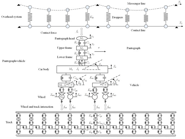
Figure 1. Vertical coupling model for overhead system-pantograph-vehicle-track system.
2.1. Modeling of overhead system
The overhead system is comprised of three main components. The contact line is responsible for providing the electrical energy through a pantograph to the high-speed train. In this paper, the finite element method widely used to address complex engineering systems[25-28] is adopted here to model the overhead system. The messenger line and droppers are used to support the contact line. The contact and messenger lines are discretized as a number of nonlinear cable elements according to the concept of the finite element method. Figure 2 presents a segment of the nonlinear cable with an unstrained length of
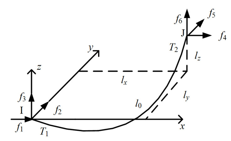
Figure 2. Nonlinear cable element.
in which
By differentiating both sides of Equation (1), the flexibility stiffness can be obtained.
where
where
It is worth noting that, after the initial configuration is determined, the initial length
Droppers only can work in tension and have no resistance to compression force, which behave as one-sided trusses. In this paper, a similar approach is adopted to derive the stiffness matrix of a truss element. Then, a shape-finding method is adopted to calculate the initial configuration of the overhead system, which has been verified by several numerical examples[29]. After the initial configuration is determined, a nonlinear finite element dynamic analysis is performed to solve the dynamic response of the overhead system. The global stiffness matrix
where
2.2. Modeling of pantograph-vehicle
As shown in Figure 1, the pantograph-vehicle is modeled as a multi-rigid-body system with 13 DOFs (degrees of freedom). Apart from the vertical motion, the rolling motions of the car body
where
where
2.3. Modeling of track
The railway track is modeled by the Euler-Bernoulli beam supported by elastic foundations, comprised of the sleepers and ballasts. The equation of motion for the rail can be written as
where
where
where
with
where
By substituting Equations (11)-(16) into Equation (10), the equation of motion for track can be obtained as
where
2.4. Contact model
The sliding contact between the pantograph and the contact line is implemented by the penalty method, in which the contact is defined through an assumption of a contact stiffness. The contact force is calculated based on a penalization of the interpenetration between the pantograph head and the contact line. The contact force is expressed as[32, 33]
where
The contact interface between the vehicle and track is between the wheel and the rail, which exhibits significant nonlinearity. The nonlinear contact can be described by Hertzian nonlinear theory of elasticity. The wheel-rail contact force can be calculated through the following equation[34]:
where
2.5. Verification of the model
It is difficult to find measurement data or a proper standard to validate the whole coupling dynamics model. The whole model is divided into the pantograph-overhead system model and the vehicle-track model. The validation of each model is made independently. In[12], the pantograph-overhead system model is verified through a series of numerical examples. Here, the parameters of pantograph and overhead system in EN 50318[35] are adopted to undertake the simulation using the presented model. The statistics of the simulation results are listed in Table 1 according to EN 50318. It can be found that the simulation results show excellent agreements with the requirements of EN 50318. Thus, the pantograph and overhead system model are thought to be valid.
Validation of the pantograph and overhead system mode according to EN 50318
| Speed | 275 [km/h] | |||
| Pantograph | 1 | 2 | ||
| Range of acceptance | Result | Range of acceptance | Result | |
| 141.5-146.5 | 143.1 | 141.5-146.5 | 144.4 | |
| 31.9-34.8 | 33.3 | 50.0-54.5 | 51.6 | |
| 26.4-28.9 | 27.2 | 41.2-45.4 | 42.8 | |
| 16.2-22.4 | 19.3 | 25.2-34.7 | 29.3 | |
| 211.9-244 | 222.9 | 241-290 | 260.4 | |
| 71-86 | 85.8 | 14-50 | 34.5 | |
| Speed | 320 [km/h] | |||
| Pantograph | 1 | 2 | ||
| Range of acceptance | Result | Range of acceptance | Result | |
| 166.5-171.5 | 169.4 | 166.5-171.5 | 168.8 | |
| 49.5-62.9 | 53.7 | 30.2-43.8 | 42.3 | |
| 38.7-44.4 | 40.1 | 14.3-23.3 | 19.0 | |
| 29.0-46.2 | 35.7 | 29.0-46.2 | 37.9 | |
| 295-343 | 295.0 | 252-317 | 269.5 | |
| 55-82 | 60.0 | 51-86 | 59.7 | |
For the validation of the vehicle-track model, the high-speed vehicle-track parameters listed in Table 2 and Table 3 are adopted[34]. The simulation results are compared with the results of the Zhai model, which is a simulation method for the vertical interactions between cars and tracks based on the well-known Zhai method[34]. Consider in the simulation that the vehicle speed is 300 km/h and the wavelength and wave depth of rail irregularity are 10 m and 0.5 mm, respectively. Figure 3A shows the displacement of the car body calculated from the presented model and the Zhai model. The results of the wheel displacement are compared in Figure 3B. It can be observed that the numerical results of the two models are only slightly different. Therefore, the present vehicle-track interaction model is considered valid.
Parameters of the high-speed vehicle
| Car body mass (kg) | 52000 |
| Car body pitch moment of inertia (kg m | 2.31 |
| Bogie mass (kg) | 3200 |
| Bogie pitch moment of inertia (kg m | 3120 |
| Wheelset mass (kg) | 1400 |
| Primary suspension stiffness (N/m) | 1.87 |
| Primary suspension damping (N s/m) | 5 |
| Secondary suspension stiffness (N/m) | 1.72 |
| Secondary suspension damping (N s/m) | 1.96 |
| Distance between two bogie centers (m) | 18 |
| Distance between two axles of the same bogie (m) | 2.5 |
| Wheel rolling radius (m) | 0.4575 |
Parameters of the high-speed track
| Elastic modulus of rail (N/m | 2.059 |
| Area moment of rail cross-section (m | 3.217 |
| Rail mass per unit length (kg/m) | 60.64 |
| Mass of half sleeper (kg) | 170 |
| Rail pad stiffness (N/m) | 6.0 |
| Rail pad damping (N s/m) | 7.5 |
| Sleeper spacing (m) | 0.6 |
| Effective support length of half sleeper (m) | 1.175 |
| Sleeper width (m) | 0.277 |
| Ballast density (kg/m | 1.9 |
| Elastic modulus of ballast (Pa) | 1.2 |
| Damping of ballast (N s/m) | 6.0 |
| Shear stiffness of ballast (N/m) | 7.84 |
| Shear damping of ballast (N s/m) | 8.0 |
| Ballast stress distribution angle ( | 35 |
| Ballast thickness (m) | 0.35 |
| Subgrade K | 1.9 |
| Damping of subgrade (N s/m) | 1.0 |
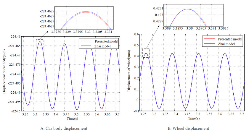
Figure 3. Verification of the vehicle-track model.
3. NUMERICAL ALGORITHMS
In this section, an interactive algorithm is proposed to couple the two sub-models. Therefore, there are three main interactive procedures in this solution algorithm. Two of them are used to deal with the nonlinear wheel-track dynamic interaction and the pantograph-overhead system dynamic interaction. The third is used to deal with the nonlinear behavior of each dropper working in tension or compression, as well as update the stiffness matrix of each cable element of messenger/contact line. The iterative procedure for the whole coupled system in each time step (from
Step 1. Calculate the contact points of the pantograph-overhead system interaction and the vehicle-track interaction.
Step 2. Initialize the iteration count
Step 3. Update the wheel-track forces
Step 4. Exert the wheel-track forces
Step 5. Update the wheel-track forces
Step 6. Exert the wheel-track force
Step 6-1. Initialize the iteration count
Step 6-2. Calculate the contact force
Step 6-3. Update the nodal forces
Step 6-3-1. Calculate
Step 6-3-2. Initialize the internal force vector
Step 6-3-3. Calculate the relative positions
Step 6-3-4. Calculate
Step 6-3-5. Calculate the correction vector of internal forces
Step 6-3-6. Update the internal forces
Step 6-4. Update the nodal forces
Step 6-5. Formulate the internal force vector
Step 6-6. Use the internal force vector
Step 6-7. Formulate the global stiffness matrix
Step 6-8. Exert the incremental excitation vector
Step 6-9. Update the displacement vector
Step 6-10. Exert the pantograph-overhead system contact force
Step 6-11. Check the convergence of the incremental displacement vectors
Step 6-12. Update the iteration count
Step 7. Check the convergence of the incremental displacement vector
Step 8. Update the acceleration vectors and velocity vectors of overhead system, track, and vehicle-track systems according to Newmark method. Enter the next time step
It should be noted that the mass of vehicle is several orders of magnitude higher than the pantograph, and the effect of pantograph vibration on the car body can be neglected. In this work, we investigate the pantograph-overhead system interaction with the perturbations of vehicle-track and achieve an accurate simulation result. This interaction between the pantograph and the vehicle is also considered in the simulation. As indicated in[36], the choice of numerical integrator and the time-space discretization has a significant effect on the numerical results. In this paper, the frequency of interest is limited to 0-20 Hz. A high sampling frequency of 2000 Hz is adopted in the numerical simulation to ensure numerical stability. The element size in the contact wire is set as 0.25 m to ensure that numerical error cannot affect the results in the frequency range of interest.
4. NUMERICAL ANALYSIS
To reveal the influence of the vehicle-track vibration on the pantograph-overhead system interaction, a whole coupled dynamics model for the railway system is established according to the description in Section 2. The parameters of a high-speed overhead system constructed in China are adopted, as shown in Figure 4A. The lumped parameters of the DSA-380 pantograph are given in Figure 4B. The parameters in Table 1 and Table 2 are adopted for the high-speed vehicle-track model. The flow chart of the subsequent analysis is presented in Figure 5.
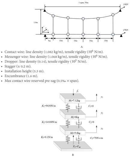
Figure 4. Parameters of the pantograph-overhead system: (A) geometry information of a simple overhead system model; and (B) three-DOF model of a pantograph.
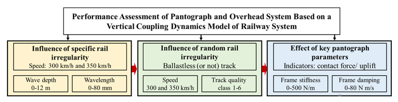
Figure 5. Flow chart of analysis in this paper.
4.1. Influence of specific rail irregularity
This section mainly focuses on the analysis of the influence of the rail irregularity with specific wavelength and wave depth on the pantograph-overhead system interaction. The rail irregularity can be described as[37]
where
The response of the high-speed overhead system-pantograph-vehicle-track is solved by employing the iterative algorithms proposed in Section 3.
The resulting contact force of the pantograph-overhead system with different wave depths of rail irregularity is shown in Figure 6A-D, in which the vehicle speeds are 300 and 350 km/h and the wavelengths of rail irregularity are 15 and 60 mm, respectively. All the results of contact force are filtered in the frequency range of interest from 0 to 20 Hz. It can be observed that the increase of the wave depth of rail irregularity leads to a significant increase of the fluctuation in contact force between the pantograph and the overhead system. When the wave depth increases from 0 to 8 mm, the waveforms of the contact force are similar at the two different vehicle speeds, while the fluctuation in contact force increases. However, when the irregularity wave depth increases up to 12 mm, the waveform of contact force undergoes a big change and a bigger fluctuation in contact force can be observed. In particular, at the wave depth of 12 mm, contact loss can be found and the maximum contact force reaches 380 N in Figure 6A. The overall maximum value of contact force appears in Figure 6C, which reaches more than 420 N.
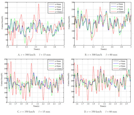
Figure 6. Results of contact force at different wave depths of rail irregularity.
The corresponding results of the pantograph head uplift and the contact wire deflection at contact point are shown in Figure 7A-D and Figure 8A-D, respectively. The structural characteristics of the overhead system can be observed obviously from the vibration of the pantograph head, as well as the displacement of the contact wire. Similar to the contact force, the vibrations of the pantograph head and the contact wire also experience continuous increases with the increase of the wave depth of rail irregularity. The minimum values of the pantograph head uplift and the contact wire deflection appear in Figure 7A and Figure 8A, respectively, when the irregularity wave depth increases to 12 mm at a vehicle speed of 300 km/h. The maximum values appear in Figure 7C and Figure 8C at a vehicle speed of 350 km/h and an irregularity wavelength of 15 mm.
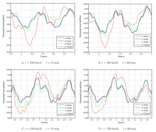
Figure 7. Results of pantograph head uplift at different wave depths of rail irregularity.
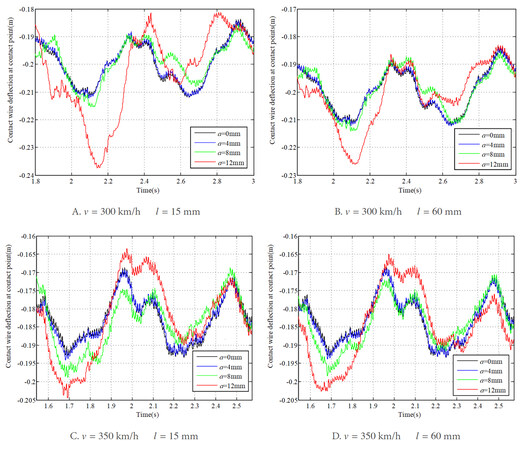
Figure 8. Results of contact wire deflection at contact point at different wave depths of rail irregularity.
To evaluate the influence of the rail irregularity wave depth on the current collection of the pantograph-overhead system, the standard deviation of contact force is shown in Figure 9 at different wave depths of rail irregularity. It is found that the standard deviation increases continuously with the increase of the wave depth of rail irregularity. Especially when it reaches 6 mm, the standard deviation shows a sharp increase. It can be concluded that the increase of the wave depth of the rail irregularity can lead to a significant increase of the fluctuation in contact force, which may result in the deterioration of current collection of the pantograph-overhead system.
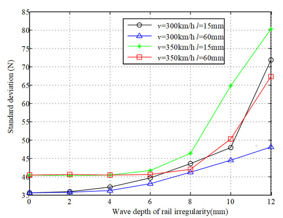
Figure 9. Standard deviation and statistical minimum value of contact force at different wave depths of rail irregularity.
Apart from the analysis of the dynamic performance at wave depths of rail irregularity, the following investigation mainly focuses on revealing the influence of the wavelength of rail irregularity on the pantograph-overhead system interaction. Suppose that the wave depth of rail irregularity is 10 mm, and the vehicle speeds are 300 and 350 km/h, respectively. The results of the contact force with different wavelengths of rail irregularity are shown in Figure 10A, B. It is found that, although the wave depth of rail irregularity remains unchanged, the contact force changes with the wavelength of rail irregularity at each vehicle speed.
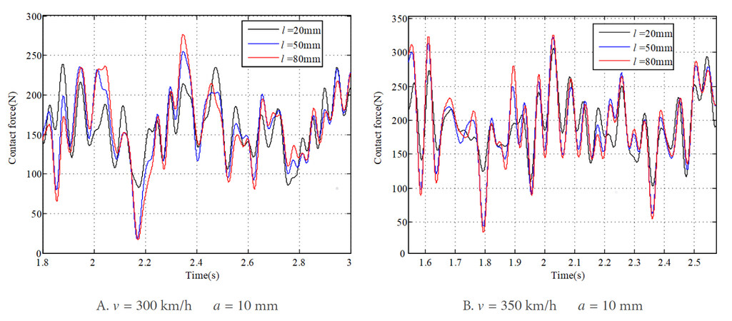
Figure 10. Results of contact force at different wavelengths of rail irregularity.
The corresponding results of the pantograph head uplift and the contact wire deflection are shown in Figure 11A, B and Figure 12A, B, respectively. The difference in the dynamic response with different wavelengths of rail irregularity can be observed obviously. The vibrations of the pantograph head and contact wire are different at different wavelengths of rail irregularity. The results of the standard deviation of contact force at different wavelengths of rail irregularity are plotted in Figure 13. It can be observed that the standard deviation changes much with different wavelengths of rail irregularity. Generally, the trends of the standard deviation with respect to the irregularity wavelength at different vehicle speeds are similar. The maximum value reaches 55.6 and 47.9 N with the same irregularity wavelength of 80 mm at vehicle speeds of 350 and 300 km/h, respectively. The overall minimum value of the standard deviation of contact force can be found in the case with the irregularity wavelength of 20 mm, which may ensure a relatively good current collection quality for the pantograph-overhead system. Thus, it can be concluded that both the wave depth and wavelength of rail irregularity seriously affect the interaction performance. Therefore, it is necessary to include them in the simulation and design of overhead system-pantograph for high-speed trains. It is also important to determine any rail irregularity wavelength that is detrimental to the current collection, which should be investigated in the future.
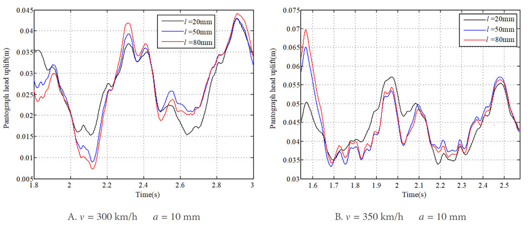
Figure 11. Results of pantograph head uplift at different wavelengths of rail irregularity.
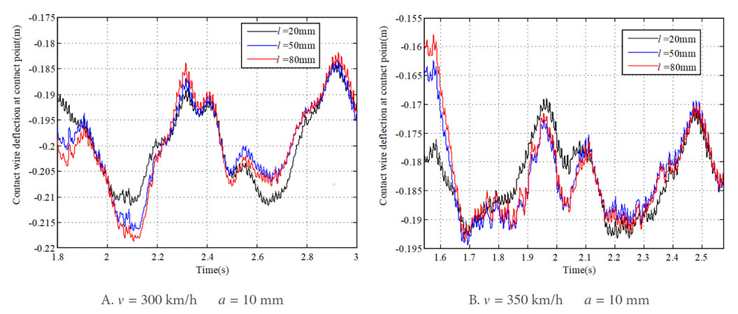
Figure 12. Results of contact wire deflection at contact point at different wavelengths of rail irregularity.

Figure 13. Results of standard deviation of contact force at different wavelengths of rail irregularity.
It is well known that rail irregularity can lead to vibration of the car body. Figure 14A shows the displacement of the car body with the rail irregularity wavelength of 15 mm and wave depth of 10 mm at a vehicle speed of 300 km/h. A spectral estimation method is utilized to analyze the frequency characteristics, as shown in Figure 14B. The spatial frequency with the highest power appears at 0.067 m
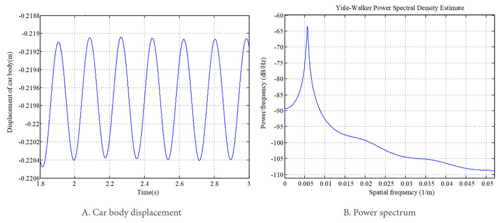
Figure 14. Car body displacement and its power spectrum.
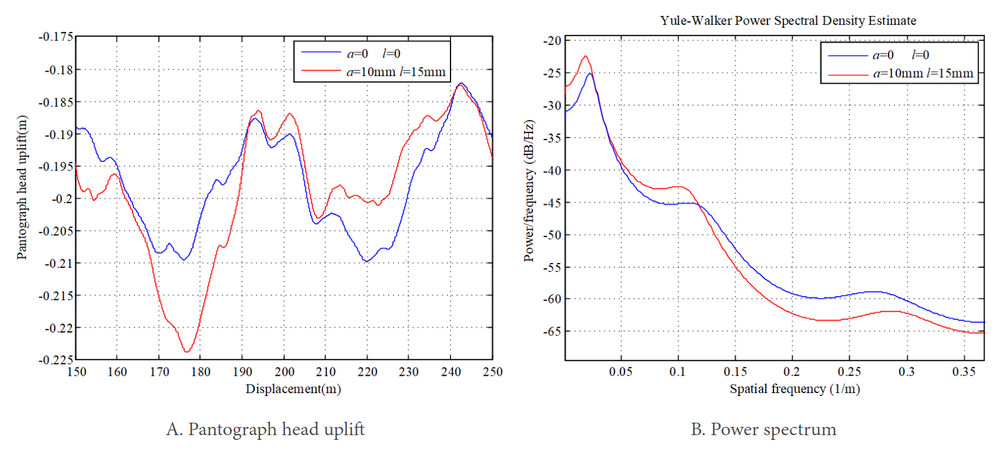
Figure 15. Pantograph head uplift and its spectral estimation.
4.2. Influence of random rail irregularity
The irregularity of a real track can be considered a random variable. In this section, the random rail irregularity is included in the track model, and its influence on the pantograph-overhead system interaction is studied. The track irregularity can be split up from the lowest (1) to the highest (6) quality classes[24] to study the dynamics of pantograph and overhead system interaction. The PSD function of the rail irregularity with different levels is presented in Table 4. The results of the contact force, pantograph head uplift, and contact wire deflection with different types of track irregularity are shown in Figures 16-18, respectively. Figure 16 shows that the contact force with the lowest-quality track fluctuates more compared with the others at each vehicle speed. A similar conclusion can be obtained for pantograph head uplift and contact wire deflection [Figure 17 and Figure 18]. The vibrations of the contact wire and the pantograph head with the lowest-quality track are significantly larger than others, which may exert a negative influence on the current collection. It is obvious that, due to the low quality of track, not only the maximum values of the vertical displacements of pantograph head and contact wire increase, but also the minimum values decrease.
Coefficients of rail irregularities with different rail levels
| Coefficient | Rail quality level | ||||||
| 1 | 2 | 3 | 4 | 5 | 6 | ||
| PSD of rail irregularity | 16.72 | 9.53 | 5.29 | 2.96 | 1.67 | 0.95 | |
| 2.33 | 2.33 | 2.33 | 2.33 | 2.33 | 2.33 | ||
| 1.31 | 1.31 | 1.31 | 1.31 | 1.31 | 1.31 | ||
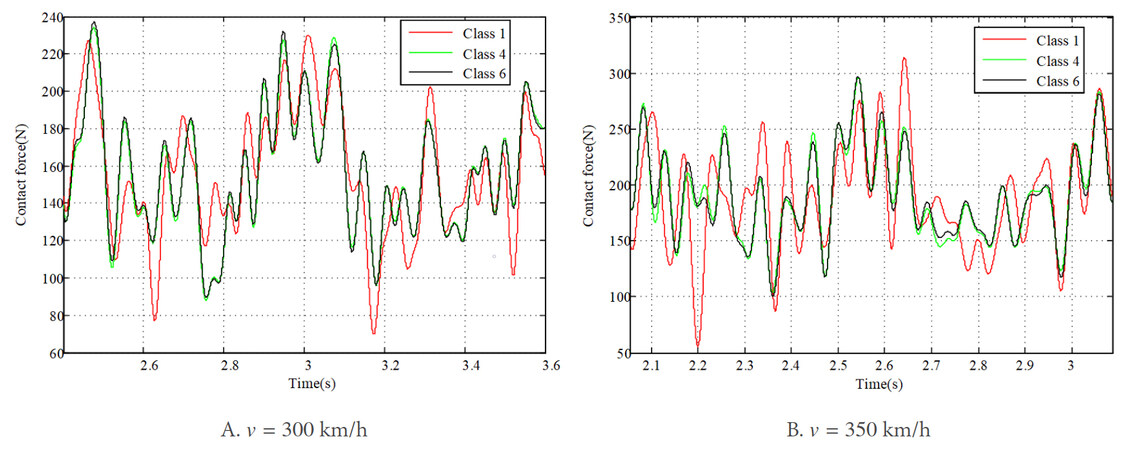
Figure 16. Results of contact force with different types of track irregularities.
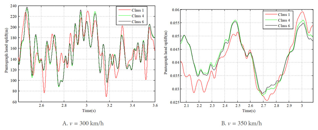
Figure 17. Results of pantograph head uplift with different types of track irregularities.
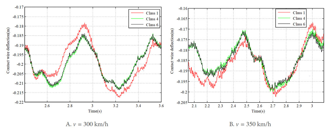
Figure 18. Results of contact wire deflection at contact point with different types of track irregularities
The results of standard deviation of contact force with different qualities of track irregularities at vehicle speeds of 300 and 350 km/h are shown in Figure 19. It can be observed that the fluctuation in contact force shows a continuous decrease with the improvement of the rail quality. For the quality class of 2-6, the standard deviation of contact force does not experience a significant change, which means that the influence of the random track irregularity is not as significant as the track irregularity with specific wave depth and wavelength. This conclusion is consistent with that found in[24].
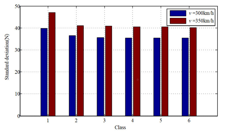
Figure 19. The results of standard deviation of contact force with different qualities of track irregularities.
Ballastless track is widely used in modern high-speed railway systems, in which the elasticity of track is mainly provided by the rail pad, as shown in Figure 20. This kind of track is designed to ensure a more stable operation of high-speed vehicles compared with the traditional track. Hence, the influence of the vehicle-ballastless track vibration on the pantograph-overhead system dynamic response is investigated compared with the traditional track. Consider that the quality level of track irregularities is 1 and the vehicle speeds are 300 and 350 km/h, respectively.
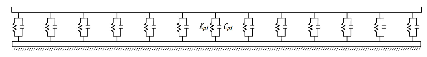
Figure 20. Ballastless track.
The results of contact force calculated with the traditional track and the ballastless track are compared in Figure 21. It can be observed that, at each vehicle speed, the results of contact force calculated with different kinds of tracks do not exhibit a large difference. However, by comparing the results of the pantograph head uplift [Figure 22], as well as the contact wire deflection at contact point [Figure 23], one can observe that the ballastless track can reduce the vibration of the pantograph head and the contact wire slightly. The standard deviations of contact force with the traditional track and the ballastless track are compared in Figure 24. They experience slight decreases of 0.26 and 0.43 N at 300 and 350 km/h, respectively, when the ballastless track is used. Thus, the ballastless track can make a small contribution to improving the current collection quality for high-speed pantograph-overhead system, in comparison with the traditional track.
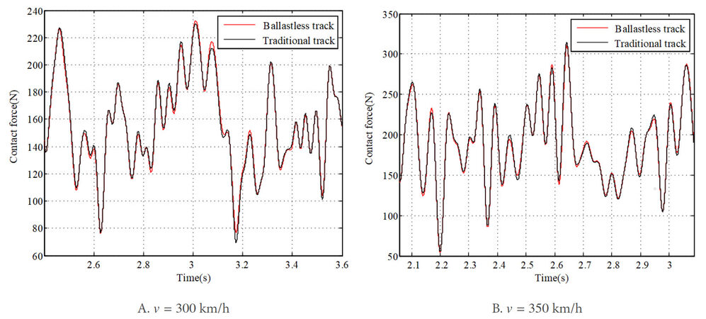
Figure 21. Comparison of contact force between traditional tack and ballastless track.
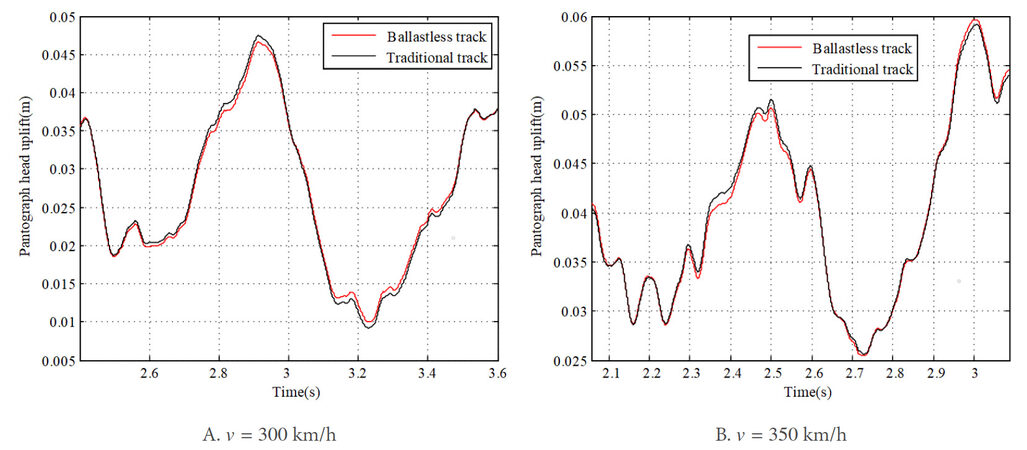
Figure 22. Comparison of pantograph head uplift between traditional tack and ballastless track.
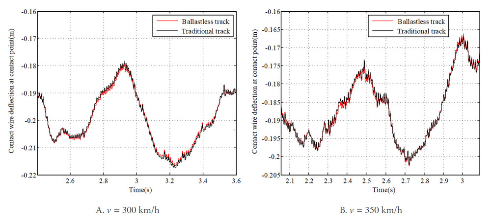
Figure 23. Comparison of contact wire deflection at contact point between traditional tack and ballastless track.
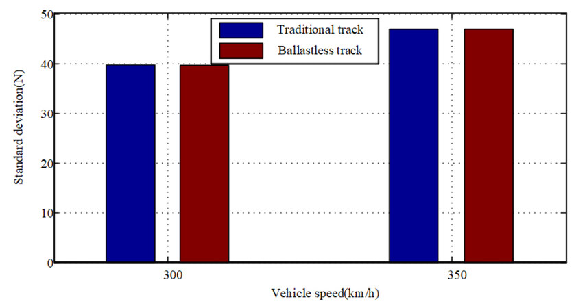
Figure 24. Results of standard deviation of contact force with traditional tack and ballastless track.
The lower frame stiffness
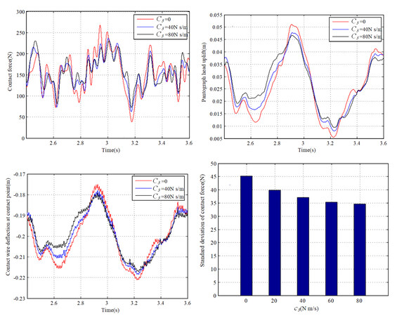
Figure 25. Results of the pantograph and overhead system dynamic response with different
The results of dynamic response with different
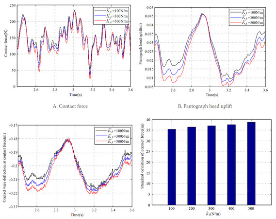
Figure 26. Results of the pantograph-overhead system dynamic response with different
5. CONCLUSIONS
This paper mainly focuses on the analysis of the influence of vehicle-tack vibration on the dynamic behavior of the pantograph-overhead system for the modern high-speed railway. A whole coupling model of railway system is established. A numerical algorithm for solving the coupled model is proposed, which is realized by the combination of the nonlinear finite element procedure for the pantograph-overhead system and the solution procedure for the vehicle-track dynamics. The influence of the vehicle-track vibration on the pantograph-overhead system interaction is studied through several numerical examples. The conclusions can be summarized as follows:
(1) The increase of the track irregularity wave depth leads to the increase of the fluctuation in contact force and the vibration of the pantograph-overhead system, which may aggravate the current collection.
(2) The wavelength of track irregularity exerts a noticeable effect on the dynamic behavior of pantograph-overhead system. It is necessary to find the wavelength of track irregularity which is detrimental to the current collection in future works.
(3) The frequency characteristics of the rail irregularity can be detected from the car body response significantly, which cannot be observed from the power spectrum of the dynamic response of the pantograph head uplift.
(4) A higher-quality track is more beneficial to the pantograph-overhead system current collection compared to a lower-quality track.
(5) The use of the ballastless track can slightly improve the current collection of the pantograph-overhead system.
(6) The increase of
It should be noted that the lumped mass model of the pantograph used in this paper is a physical representation of the first several critical modes of a realistic one. The adopted model can only consider the effect of very low-frequency effect of vehicle-track vibration on the pantograph-overhead system interaction. A multibody dynamics model that fully describes the geometrical configuration of a pantograph is desired to capture a more realistic effect of vehicle-track perturbations on the pantograph-catenary system.
DECLARATIONS
Authors' contributions
Made substantial contributions to conception and design of the study and performed data analysis and interpretation: Song Y
Performed data acquisition, as well as providing administrative and simulation support: Duan F
Availability of data and materials
Not applicable.
Financial support and sponsorship
This study was partly supported by the National Natural Science Foundation of China (52102478), and Norwegian Railway Directorate.
Conflicts of interest
All authors declared that there are no conflicts of interest.
Ethical approval and consent to participate
Not applicable.
Consent for publication
Not applicable.
Copyright
©The Author(s) 2022.
REFERENCES
1. Li Z, Chen J, Deng J. A feedforward air-conditioning energy management method for high-speed railway sleeper compartment. Complex Eng Syst 2022:2.
2. Lu Z, Wang X, Yue K, Wei J, Yang Z. Coupling model and vibration simulations of railway vehicles and running gear bearings with multitype defects. Mech Mach Theory 2021;157:104215.
3. Wang C, Zhang Q, Li H, Zhang L, Zhang B. Warpage deformation behavior of metal laminates. Chinese J Eng 2021;43:409-21.
4. Tang W, Ma H, Yuan Y, Liu Z, Yu Z. Investigation on the influence of Cu-Al2O3 dispersion copper high-speed railway contact wire on current-collecting quality of pantograph-catenary. J Railw Sci Eng 2021;18:1098-104.
5. Luo L, Ye W, Wang J. Defect detection of the puller bolt in high-speed railway catenary based on deep learning. J Railw Sci Eng 2021;18:605-14.
6. Gao SB, Liu ZG, Yu L. Detection and monitoring system of the pantograph-catenary in high-speed railway (6C). In 2017 7th international conference on power electronics systems and applications - smart mobility, power transfer & security (PESA), Hong Kong, China, 12-14 December 2017; pp. 1-7.
7. Xu Z, Gao G, Yang Z, Wei W, Wu G. An online monitoring device for pantograph catenary arc temperature detect based on atomic emission spectroscopy. In 2018 IEEE international conference on high voltage engineering and application (ICHVE) 2018; pp. 1-4.
8. Zhang Y, Yue Y, Zhao S, Sihua W. Research on galloping response of catenary positive feeder in gale area considering surface roughness of stranded wire. J Railw Sci Eng 2021;18:1885-94.
9. Song Y, Liu Z, Wang H, Lu X, Zhang J. Nonlinear analysis of wind-induced vibration of high-speed railway catenary and its influence on pantograph - catenary interaction. Veh Syst Dyn 2016;54:723-47.
10. Zhang W, Zou D, Tan M, Zhou N, Li R, Mei G. Review of pantograph and catenary interaction. Front Mech Eng 2018;13:311-22.
11. Liu Z, Song Y, Han Y, Wang H, Zhang J, Han Z. Advances of research on high-speed railway catenary. J Mod Transp 2018;26:1-23.
12. Song Y, Liu Z, Wang H, Lu X, Zhang J. Nonlinear modelling of high-speed catenary based on analytical expressions of cable and truss elements. Veh Syst Dyn 2015;53:1455-79.
13. Yao Y, Zhou N, Mei G, Zhang W. Dynamic Analysis of Pantograph-Catenary System considering Ice Coating. Shock Vib 2020:1-15.
14. Tur M, García E, Baeza L, Fuenmayor FJ. A 3D absolute nodal coordinate finite element model to compute the initial configuration of a railway catenary. Eng Struct 2014;71:234-43.
15. Bautista A, Montesinos J, Pintado P. Dynamic interaction between pantograph and rigid overhead lines using a coupled FEM - Multibody procedure. Mech Mach Theory 2016;97:100-11.
16. Lu X, Liu Z, Song Y, Wang H, Zhang J, Wang Y. Estimator-based multiobjective robust control strategy for an active pantograph in high-speed railways. J Rail Rapid Transit 2018;232:1064-77.
17. Gregori S, Tur M, Nadal E, Fuenmayor FJ. An approach to geometric optimisation of railway catenaries. Veh Syst Dyn 2018;56:1162-86.
18. Wang W, Liang Y, Zhang W, Iwnicki S. Effect of the nonlinear displacement-dependent characteristics of a hydraulic damper on high-speed rail pantograph dynamics. Nonlinear Dyn 2019;95:3439-64.
19. Liu Z, Liu W, Han Z. A high-precision detection approach for catenary geometry parameters of electrical railway. IEEE Trans Instrum Meas 2017;66:1798-808.
20. Han Y, Liu Z, Geng X, Zhong J. Fracture Detection of Ear Pieces in Catenary Support Devices of High-speed Railway Based on HOG Features and Two-Dimensional Gabor Transform. J China Railw Soc 2017;39:52-7.
21. Liu W, Liu Z, Li Y, Wang H, Yang C, Wang D, Zhai D. An automatic loose defect detection method for catenary bracing wire components using deep convolutional neural networks and image processing. IEEE Trans Instrum Meas 2021;70:1-14.
22. Cheng H, Wang J, Liu J, Cao Y, Li H, Xu X. Comprehensive evaluation method of catenary status based on improved multivariate statistical control chart. J Railw Sci Eng 2021;18:3048-56.
23. Wang H, Nunez A, Liu Z, Zhang D, Dollevoet R. A Bayesian Network Approach for Condition Monitoring of High-Speed Railway Catenaries. IEEE Trans Intell Transp Syst 2020;21:4037-51.
24. Song Y, Wang Z, Liu Z, Wang R. A spatial coupling model to study dynamic performance of pantograph-catenary with vehicle-track excitation. Mech Syst Signal Process 2021;151:107336.
25. Ma H, Zhang D, Yi Y. Influence of the soft reduction process on the sensitivity of the inner crack in heavy rail steel bloom. Chinese J Eng 2021;43:1679-88.
26. Qin R, Zhu B, Qiao K, Wang D, Sun N, Yuan X. Simulation study of the protective performance of composite structure carbon fiber bulletproof board. Chinese J Eng 2021;43:1346-54.
27. Bruni S, Ambrosio J, Carnicero A, et al. The results of the pantograph-catenary interaction benchmark. Veh Syst Dyn 2015;53:412-35.
28. Zhang M, Xu F. Tuned mass damper for self-excited vibration control: Optimization involving nonlinear aeroelastic effect. J Wind Eng Ind Aerodyn 2022;220:104836.
29. Yang J, Song Y, Lu X, Duan F, Liu Z, Chen K. Validation and Analysis on Numerical Response of Super-High-Speed Railway Pantograph-Catenary Interaction Based on Experimental Test. Shock Vib 2021;2021:1-13.
30. Zhai W, Wang K, Cai C. Fundamentals of vehicle-track coupled dynamics. Veh Syst Dyn 2009;47:1349-76.
31. Ouyang H. Moving-load dynamic problems: A tutorial (with a brief overview). Mech Syst Signal Process 2011;25:2039-60.
32. Lopez-Garcia O, Carnicero A, Maroño JL. Influence of stiffness and contact modelling on catenary-pantograph system dynamics. J Sound Vib 2007;299:806-21.
33. Ye Y, Huang P, Sun Y, Shi D. MBSNet: A deep learning model for multibody dynamics simulation and its application to a vehicle-track system. Mech Syst Signal Process 2021;157:107716.
34. Zhai W. Vehicle-track coupled dynamics models Beijing: Science Press; 2020.
35. European Committee for Electrotechnical Standardization. EN 50318. Railway applications - current collection systems - validation of simulation of the dynamic interaction between pantograph and overhead contact line. Brussels: European Standards (EN), 2018.
36. Sorrentino S, Anastasio D, Fasana A, Marchesiello S. Distributed parameter and finite element models for wave propagation in railway contact lines. J Sound Vib 2017;410:1-18.
37. Wu TX, Thompson DJ. On the parametric excitation of the wheel/track system. J Sound Vib 2004;278:725-47.
38. Ambrósio J, Pombo J, Pereira M. Optimization of high-speed railway pantographs for improving pantograph-catenary contact. Theor Appl Mech Lett 2013;3:013006.
39. Pombo J, Ambrósio J. Influence of pantograph suspension characteristics on the contact quality with the catenary for high speed trains. Comput Struct 2012;110:32-42.
Cite This Article
Export citation file: BibTeX | RIS
OAE Style
Song Y, Duan F. Performance assessment of pantograph and overhead system based on a vertical coupling dynamics model of the railway system. Complex Eng Syst 2022;2:9. http://dx.doi.org/10.20517/ces.2022.09
AMA Style
Song Y, Duan F. Performance assessment of pantograph and overhead system based on a vertical coupling dynamics model of the railway system. Complex Engineering Systems. 2022; 2(2): 9. http://dx.doi.org/10.20517/ces.2022.09
Chicago/Turabian Style
Song, Yang, Fuchuan Duan. 2022. "Performance assessment of pantograph and overhead system based on a vertical coupling dynamics model of the railway system" Complex Engineering Systems. 2, no.2: 9. http://dx.doi.org/10.20517/ces.2022.09
ACS Style
Song, Y.; Duan F. Performance assessment of pantograph and overhead system based on a vertical coupling dynamics model of the railway system. Complex. Eng. Syst. 2022, 2, 9. http://dx.doi.org/10.20517/ces.2022.09
About This Article
Copyright

Data & Comments
Data


 Cite This Article 11 clicks

 Like This Article 31
likes
Like This Article 31
likes


Comments
Comments must be written in English. Spam, offensive content, impersonation, and private information will not be permitted. If any comment is reported and identified as inappropriate content by OAE staff, the comment will be removed without notice. If you have any queries or need any help, please contact us at support@oaepublish.com.