Download PDF
Research Article  |  Open Access  |  26 Dec 2022

Stability analysis for highly nonlinear switched stochastic systems with time-varying delays

Views: 1288 |  Downloads: 741 |  Cited:   1
Complex Eng Syst 2022;2:17.
10.20517/ces.2022.48 |  © The Author(s) 2022.
Author Information
Article Notes
Cite This Article

Abstract

In this paper, we examine the stability of highly nonlinear switched stochastic systems (SSSs) with time-varying delays, where the switching time instants are deterministic rather than stochastic. Herein, the boundedness of the global solution is first proven for highly nonlinear SSSs via the average dwell time (ADT) method and multiple Lyapunov function (MLF) approach. Then, the stability criteria for qth moment exponential stability and almost surely exponential stability are presented. The main difficulty lies in the presence of switching and time-varying delay terms, which prevents the validation of existing methods. New inequality techniques have been developed to counteract the effects of switching signals and time-varying delays. Finally, an example is provided to verify the effectiveness of the results.

Keywords

Highly nonlinear switched stochastic systems, deterministic switching signal, time-varying delays, average dwell time, multiple Lyapunov function

1. INTRODUCTION

Switched systems are important dynamic systems. The idea of switching has been widely applied in various fields, such as aircraft attitude control [1], ecological dynamics [2], and financial markets [3]. With the increasing complexity of system architectures, dynamical analysis of switched systems has attracted significant academic interest. A switched system consists of a family of continuous-time dynamics, discrete-time dynamics, and switching rules between subsystems. According to the switching signal features, switched systems are divided into two categories, {namely}, deterministic switched systems and randomly switched systems. Many researchers have focused on stabilization and stability analyses of various switched systems. For example, in [4], a series of results on stochastic differential equations (SDEs) with Markovian switching was obtained. In particular, the authors have provided some useful stability criteria. In [5], the authors studied the input-to-state stability of time-varying switched systems by employing the ADT method coupled with the MLF approach. The authors of [6] investigated the stability of switched stochastic delay neural networks with all unstable subsystems based on discretized Lyapunov-Krasovskii functions (DLKFs). In [7], a novel Lyapunov function was designed to ensure a non-weighted $$ \mathcal{L}_2 $$ gain for switched systems with asynchronous switching. In[8], a hidden Markov model was proposed to study the finite region $$ H_\infty $$ asynchronous control problem for two-dimensional Markov jump systems. Other interesting researches on switched systems can be found in [9-11] and references therein.

The linear growth condition (LGC) is crucial for ensuring the existence of a global solution for a stochastic system. However, many stochastic systems do not satisfy LGC. Hence, the solution of a stochastic system may explode in a finite time. Recently, the stability of stochastic systems without LGC has drawn considerable attention. For instance, the authors of [12] investigated the stability and boundedness of nonlinear hybrid stochastic differential delay equations without LGC based on a Lyapunov function approach. By introducing a polynomial growth condition (PGC), [13] discussed the stabilization problem of highly nonlinear hybrid SDEs. The input-to-state practically exponential stability in the sense of mean square was introduced in [14]. Sufficient conditions for stability have been obtained. Additionally, other meaningful results were reported in [15] and [16].

Time-delay is an important factor that affects dynamical performances of stochastic systems. By constructing a suitable Lyapunov function, the authors of [12] studied the stability and boundedness of highly nonlinear hybrid stochastic systems with a time delay. The authors of [17] used the ADT method to study the stability problem of SSSs, where the switching signals are deterministic. Based on the stability criteria for stochastic time-delay systems, the authors of [18] introduced a suitable Lyapunov-Krasovskii (L-K) functional, and discussed the global probabilistic asymptotic stability of the closed-loop system. In [19], the Razumikhin approach was presented to study the exponential stability of a class of impulsive stochastic delay differential systems. Using the piecewise dynamic gain method, the authors of [20] studied the global uniform ultimate boundedness of switched linear time-delay systems. Motivated by the aforementioned literature, the stability of highly nonlinear SSSs with time-varying delays is studied in this paper. Figure 1 shows the framework of this paper.

Stability analysis for highly nonlinear switched stochastic systems with time-varying delays

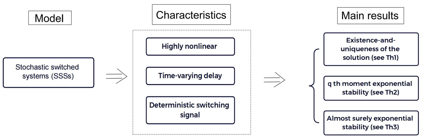
Figure 1. Framework of the paper.

The challenges of this article lie in the following two parts: (1) The time delay studied here is merely a Borel measurable function of time $$ t $$ . That is to say, it may be non-differentiable with respect to time $$ t $$ , which means that the existing methods regarding constant delays or differentiable delays are no longer applicable; (2) Rather than a Markovian switching signal, a deterministic switching signal is involved in the studied system, indicating that Markovian switched systems based M-matrix method is invalid. To address the influences of deterministic switching signals, an ADT method coupled with the MLF approach is utilized in our stability analysis.

The main advantages of this paper are as follows:

$$ (1) $$ Without the LGC, the existence and uniqueness of a global solution is proven for highly nonlinear SSSs, where a deterministic switching signal rather than a Markovian switching signal is considered.

$$ (2) $$ By integrating the ADT method and MLF approach, the $$ q $$ th moment exponential stability and almost surely exponential stability are presented for highly nonlinear SSSs with time-varying delays.

The remainder of this paper is organized as follows. An introduction of the model and important assumptions are given in Section 2. The existence of a unique global solution and stability analysis are presented in Sections 3. In Section 4, a simulation example is presented to validate our theoretical results. Finally, Section 5 concludes the paper.

Note: In this paper, $$ \mathbb{R}_{+}=(0, \infty) $$ , $$ \mathbb{N}_{+}=1, 2, \cdots, \kappa, \cdots $$ , $$ \mathbb{N}=\mathbb{N}_{+}\cup\{0\} $$ with $$ \kappa $$ being a positive finite integer, $$ \mathbb{R}^{n} $$ denotes the $$ n $$ -dimensional real space. For $$ x\in\mathbb{R}^{n} $$ , $$ |x|=\big(\sum_{i=1}^nx_i^2\big)^\frac{1}{2} $$ denotes the Euclidean norm of vector. For any matrix $$ A\in\mathbb{R}^{n\times n} $$ , $$ |A| =\sqrt{A^TA} $$ denotes the trace norm of matrix $$ A $$ , where $$ A^T $$ is the transpose of matrix $$ A $$ and $$ {\rm tr}\{A\} $$ denotes its trace. For $$ \tau>0 $$ , $$ C([-\tau, 0];\mathbb{R}^n) $$ denotes the space of all continuous functions $$ \varphi $$ from $$ [-\tau, 0]\to\mathbb{R}^n $$ with the norm $$ ||\varphi||=\sup_{-\tau\leq u\leq0}|\varphi(u)| $$ , $$ \mathcal{C}_{\mathcal{F}_0}^b([-\tau, 0];\mathbb{R}^n) $$ denotes the family of all $$ \mathcal{F}_0 $$ -measurable bounded $$ \mathcal{C}([-\tau, 0];\mathbb{R}^n) $$ -valued random variable $$ \xi=\{\xi(\theta):-\tau\leq\theta\leq0\} $$ . Let $$ (\varOmega, \mathcal{F}, \mathbb{P}) $$ be a complete probability space with a filtration $$ \{\mathcal{F}_{t}\}_{t\geq0} $$ . $$ B(t) $$ =($$ B_1(t) $$ , $$ \cdots $$ , $$ B_m(t) $$ ) denotes an $$ m $$ -dimensional $$ \mathcal{F}_t $$ -adapted Brownian motion, which is defined on a complete probability space. In addition, $$ \mathcal{V}^{1, 2} $$ denotes the family of all non-negative functions $$ V(t, x, i):[-\tau, \infty)\times\mathbb{R}^n\times\Gamma\to\mathbb{R}_+ $$ , which are first-order continuously differentiable in $$ t $$ and second-order continuously differentiable in $$ x $$ . Let $$ C([-\tau, \infty)\times\mathbb{R}^n;\mathbb{R}_+) $$ be the family of continuous functions $$ W:[-\tau, \infty)\times\mathbb{R}^n\to\mathbb{R}_+ $$ . For real numbers $$ a $$ and $$ b $$ , $$ a\wedge b=\min\{a, b\} $$ , $$ a\vee b=\max\{a, b\} $$ .

2. PRELIMINARIES

Model descriptions and assumptions are introduced in this section. In this study, we analyzed the following highly nonlinear SSS with time-varying delays:

$$ dx(t)=f_{\sigma(t)}(t, x(t), x(t-\delta_t))dt+g_{\sigma(t)}(t, x(t), x(t-\delta_t))dB(t), $$

with the initial value:

$$ \{x(t):-m\leq t\leq 0\}=\xi\in \mathcal{C}_{\mathcal{F}_0}^b([-m, 0];\mathbb{R}^{n}), $$

where $$ m>0 $$ is a constant and switching signal $$ \sigma(t):[0, \infty)\to \Gamma=\{1, 2, \cdots, \kappa\} $$ is a piecewise constant function that is continuous from the right. In particular, it is a non-random function of $$ t $$ . For $$ t\in[t_m, t_{m+1}) $$ , $$ \sigma(t)=i_m\in\Gamma $$ , where $$ t_m $$ is the $$ m $$ th switching time instant and $$ m\in\mathbb{N} $$ . For each $$ i\in\Gamma $$ , the mappings $$ f_i:\mathbb{R}^{+}\times\mathbb{R}^n\times\mathbb{R}^n\to\mathbb{R}^n $$ and $$ g_i:\mathbb{R}^{+}\times\mathbb{R}^n\times\mathbb{R}^n\to\mathbb{R}^{n\times m} $$ are Borel-measurable functions. Compared with [13], one of the merits of this paper is that the time delay $$ \delta_t $$ is merely a Borel measurable function of $$ t $$ and may be non-differentiable. Precisely, we need to impose some requirements on the time-varying delay $$ \delta_t $$ .

Assumption 1. The time-varying delay $$ \delta_t $$ is a Borel measurable function of $$ t $$ from $$ \mathbb{R}_+\to[m_1, m] $$ with the property that

$$ \bar{m}=\limsup\limits_{\Delta\to0_+} \bigg(\sup\limits_{s\geq-m}\frac{\mu(M_{s, \Delta})}{\Delta}\bigg)<\infty, $$

where $$ m_1 $$ and $$ m $$ are positive constants, $$ M_{s, \bigtriangleup}=\{t\in\mathbb{R}_+: t-\delta_t \in [s, s+\bigtriangleup)\} $$ and $$ \mu(\cdot) $$ denotes the Lebesgue measure on $$ \mathbb{R}_+ $$ .

Remark 1 Assumption 1 reveals that the time delay in SSS (1) is merely a Borel measurable function of time $$ t $$ , which means that it may be non-differentiable with respect to time $$ t $$ . In most reported studies on SSSs (see, e.g., [21-25]), the time delay $$ \delta_t $$ is always assumed to be a differentiable function and its time derivative $$ \dot{\delta}_t $$ should satisfy $$ \dot{\delta}_t\leq\bar{\delta}<1 $$ with $$ \bar{\delta} $$ being a positive constant. However, this condition is too conservative for practical application. Many time-delay functions in actual systems do not satisfy this assumption. For example, a time-varying delay $$ \delta_t $$ is defined as $$ \delta_t=0.5+0.25|\sin(10t)| $$ . If $$ \delta_t $$ is a Lipschitz continuous function with a Lipschitz coefficient $$ m_2\in (0, 1) $$ , namely, $$ |\delta_t-\delta_s|\leq m_2|t-s| $$ , then for all $$ 0\leq s. Then, $$ \delta_t $$ satisfies Assumption 1 with $$ \bar{m}=(1-m_2)^{-1} $$ . In particular, if $$ \delta_t $$ is differentiable and its derivative is bounded by $$ m_2\in (0, 1) $$ , then $$ \delta_t $$ still satisfies Assumption 1. From a theoretical perspective, a large class of functions $$ \delta_t $$ can satisfy Assumption 1. Note that the constant $$ \bar{m} $$ must not be less than $$ 1 $$ (i.e., $$ \bar{m}\geq1 $$ ). This point can be obtained from the following lemma, with $$ \psi=1 $$ .

The following lemma provides a useful inequality to obtain the stability of the SSS (1) with time-varying delays, and its proof can be found in [16].

Lemma 1[16] Let $$ T>0 $$ and $$ \psi :[t_0-m, T-m_1]\to\mathbb{R}^+ $$ be a continuous function. If Assumption 1 holds, then

$$ \int _{t_0}^{T}\psi(t-\delta_t) dt\leq \bar {m}\int_{t_0-m}^{T-m_1}\psi(t) dt. $$

The conditions for the existence and uniqueness of global solution are the local Lipschitz condition (LLC) and the LGC (see, e.g., [4, 7, 20, 26]). In this paper, the highly nonlinear SSS (1) generally does not require the LGC. Consequently, we must impose the PGC on it.

Assumption 2. (LLC & PGC) For any real number $$ b>0, i\in \Gamma $$ , there exists a constant $$ K_{b, i}>0 $$ such that

$$ |f_i(t, x, y)-f_i(t, \bar{x}, \bar{y})|\vee|g_i(t, x, y)-g_i(t, \bar{x}.\bar{y})| \leq K_{b, i} (|x-\bar{x}| + |y-\bar{y}|), $$

for all $$ x, \bar{x}, y, \bar{y}\in\mathbb{R}^n $$ , where $$ |x|\vee|\bar{x}|\vee|y|\vee|\bar{y}|\leq b $$ . Moreover, there exist constants $$ K>0, \alpha_1>1, \alpha_2\geq1 $$ such that

$$ |f_i(t, x, y)|\leq K(1+|x|^{\alpha_1}+|y|^{\alpha_1}), \\ |g_i(t, x, y)|\leq K(1+|x|^{\alpha_2}+|y|^{\alpha_2}), $$

where $$ (t, x, y)\in\mathbb{R}^{+}\times\mathbb{R}^{n}\times\mathbb{R}^{n} $$ and $$ i\in \Gamma $$ .

Assumption 3 Assume that there are two functions $$ \varLambda\in\mathcal{V}^{1, 2}([-m, \infty)\times\mathbb{R}^n\times\Gamma;\mathbb{R}_+) $$ and $$ W\in C([-m, \infty)\times \mathbb{R}^n;\mathbb{R}_+) $$ , as well as positive numbers $$ a_1, a_2, \lambda_1, \lambda_3 $$ and real numbers $$ \lambda_2, \lambda_4 $$ , satisfying $$ \lambda_1>\lambda_2, \lambda_3>\lambda_4 $$ and $$ q>2, \mu_{i}>1 $$ , such that for any $$ (t, x, y, i)\in \mathbb{R}_{+}\times\mathbb{R}^{n}\times\mathbb{R}^{n}\times\Gamma $$ ,

$$ a_1|x|^q\leq\Lambda(t, x, i)\leq a_2|x|^q, $$

$$ \varLambda(t, x, i)\leq \mu_{i}\varLambda(t, x, j), \quad \forall (t, x, i)\in\mathbb{R}_{+}\times\mathbb{R}^{n}\times\Gamma, $$

$$ \begin{array}{l} \mathcal{L}\varLambda(t, x, y, i)=\varLambda_t(t, x, i)+\varLambda_x(t, x, i)f_i(t, x, y)+\dfrac{1}{2}{\rm trace}\{{g_i}^T(t, x, y)\varLambda_{xx}(t, x, i)g_i(t, x, y)\}\\ \qquad\qquad\quad\, \, \leq-\lambda_1W(x)+\lambda_2W(y)-\lambda_3|x|^q+\lambda_4|y|^q, \end{array}$$

where $$ y=x(t-\delta_t) $$ and

$$ \begin{align*} &\varLambda_t(t, x, i)=\dfrac{\partial\varLambda(t, x, i)}{\partial t}, \\ &\varLambda_x(t, x, i)=\bigg(\dfrac{\partial\varLambda(t, x, i)}{\partial x_1}, \cdots, \dfrac{\partial\varLambda(t, x, i)}{\partial x_n}\bigg), \\ &\varLambda_{xx}(t, x, i)=\bigg(\dfrac{\partial^{2}\varLambda(t, x, i)}{\partial x_j\partial x_k}\bigg)_{n\times n}. \end{align*} $$

Moreover, assume that there exists a constant $$ \varepsilon>0 $$ , such that \\

$$ \lambda_3-\lambda_4\bar{m}e^{\varepsilon m}-\varepsilon a_{2}=0, $$

$$ \lambda_1-\lambda_2\bar{m}e^{\varepsilon m}>0. $$

Remark 2 The system studied in this research has the property of high nonlinearity. In other words, the LGC is removed from the SSS (1), which makes the considered system more general. Without the LGC, the solution of a stochastic system may explode in a finite time. To ensure the existence of a global solution, a PGC (i.e., condition (6)) is imposed on the SSS (1) (see, e.g., [13, 27, 28]). Therefore, the system (1) we studied obeys the LLC (i.e., condition (5)) and the PGC. By combining the MLF approach and ADT method, we then prove the existence and uniqueness of the global solution.

Before presenting the main results, the definition of ADT is revisited.

Definition 1[28] For a switching signal $$ \sigma(t) $$ and any $$ t\geq s\geq 0 $$ , $$ T_i(t, s) $$ and $$ N_i(t, s) $$ denote the whole running time and the switching number of the i-th subsystem over the interval $$ [s, t] $$ , respectively, $$ i\in\Gamma $$ . Then, the following inequality holds:

$$ \begin{align*} N_i(t, s)\leq\dfrac{T_i(t, s)}{\mathcal{J}_{ai}}+N_{0i}, \end{align*} $$

where $$ \mathcal{J}_{ai}>0 $$ is called the mode-dependent ADT and $$ N_{0i}>0 $$ is the mode-dependent chatter bound.

3. MAIN RESULTS

In this section, we prove the existence of a unique global solution for a highly nonlinear SSS (1) by using the ADT and MLF approaches. Then, both the $$ q $$ th moment exponential stability and almost surely exponential stability are provided for a highly nonlinear SSS (1).

Theorem 1 Under Assumptions 1-3, if there exists a constant $$ \varepsilon>0 $$ such that

$$ \mathcal{J}_{ai}>\dfrac{\ln \mu_{i}}{\varepsilon}. $$

Then, for any initial data (2), there exists a unique global solution $$ x(t) $$ for the SSS (1) on $$ [-m, \infty) $$ , and the solution satisfies

$$ \sup\limits_{-m\leq t<\infty}\textbf{E}|x(t)|^q<\infty. $$

Proof. We divide the whole proof into two steps. In step 1, for all $$ i\in\mathbb{S} $$ , we prove that the $$ i $$ -th subsystem with the initial value $$ x_i(0) $$ has a unique global solution $$ x_i(t) $$ . In step 2, when each subsystem has a unique global solution, the SSS (1) with a deterministic switching signal has a unique global solution $$ x(t) $$ on $$ [-m, \infty) $$ .

Step 1. For all $$ i\in\mathbb{S} $$ , the control system becomes

$$ dx_i(t)=f_i(t, x_i(t), y_i(t))dt+g_i(t, x_i(t), y_i(t))dB(t), \quad t\geq-m, $$

where $$ y_i(t)=x_i(t-\delta_t) $$ . Under the LLC, system (14) has a unique maximal global solution on $$ [-m, \rho_{\infty}^i) $$ , denoted as $$ x_i(t) $$ , where $$ \rho_{\infty}^i $$ is the explosion time. Then, we prove $$ \rho_{\infty}^i=\infty $$ a.s. Thus, it is necessary to define the stopping time sequence. Let $$ k_0 $$ be a constant sufficiently large to satisfy $$ k_0>|x_i(0)| $$ . For any integer $$ k\geq k_ 0 $$ , we define the stopping time sequence as follows:

$$ \begin{align*} \delta_{k, i}=\inf\{t\in[0, \rho_{\infty}^i), |x_i(t)|\geqslant k\}. \end{align*} $$

Clearly, $$ \delta_{k, i} $$ increases as $$ k\to\infty $$ and therefore we set $$ \delta_{\infty, i}:=\lim\limits_{k\to\infty}\delta_{k, i} $$ . Observe that $$ \delta_{\infty, i}\leq\rho_{\infty, i} $$ a.s. Thus, $$ \delta_{\infty, i}=\infty $$ , a.s., which yields $$ \rho_{\infty, i}=\infty $$ a.s. From the It$$ \hat{o} $$ formula and condition (9), it is easily proven that

$$ \begin{align*} &E e^{\varepsilon(t\wedge\delta_{k, i})}\Lambda(t\wedge\delta_{k, i}, x_i(t\wedge\delta_{k, i}), i)\\ &=E e^{\varepsilon t_0}\Lambda(t_0, x_i(t_0), i)+E\int_{t_0}^{t\wedge\delta_{k, i}}e^{\varepsilon s}[\varepsilon \Lambda(s, x_i(s), i)+\mathcal{L}\Lambda(s, x_i(s), i)]ds\\ &\leq E e^{\varepsilon t_0}\Lambda(t_0, x_i(t_0), i)+E\int_{t_0}^{t\wedge\delta_{k, i}}e^{\varepsilon s}[\varepsilon a_2|x_i(s)|^q-\lambda_1W(x_i(s))+\lambda_2W(y_i(s))\\ &\quad-\lambda_3|x_i(s)|^q+\lambda_4|y_i(s)|^q]ds. \end{align*} $$

By Lemma 1, we have

$$ \begin{array}{l} &E\int_{t_0}^{t\wedge\delta_{k, i}}e^{\varepsilon s}W(x_i(s-\delta_s))ds\\ &\leq e^{\varepsilon m}\bar{m}E\int_{t_0-m}^{t\wedge\delta_{k, i}}e^{\varepsilon s}W(x_i(s))ds\\ &\leq e^{\varepsilon m}\bar{m}E\int_{t_0-m}^{t_0}e^{\varepsilon s}W(x_i(s))ds+e^{\varepsilon m}\bar{m}E\int_{t_0}^{t\wedge\delta_{k, i}}e^{\varepsilon s}W(x_i(s))ds, \end{array}$$

and

$$ \begin{array}{l} &E\int_{t_0}^{t\wedge\delta_{k, i}}e^{\varepsilon s}|x_i(s-\delta_s)|^qds\\ &\leq e^{\varepsilon m}\bar{m}E\int_{t_0-m}^{t\wedge\delta_{k, i}}e^{\varepsilon s}|x_i(s)|^qds\\ &\leq e^{\varepsilon m}\bar{m}E\int_{t_0-m}^{t_0}e^{\varepsilon s}|x_i(s)|^qds+e^{\varepsilon m}\bar{m}E\int_{t_0}^{t\wedge\delta_{k, i}}e^{\varepsilon s}|x_i(s)|^qds. \end{array} $$

Hence,

$$ \begin{align*} &Ee^{\varepsilon(t\wedge\delta_{k, i})}\Lambda(t\wedge\delta_{k, i}, x_i(t\wedge\delta_{k, i}), i)\\ &\leq C-(\lambda_3-\lambda_4\bar{m}e^{\varepsilon m}-\varepsilon a_2)E\int_{t_0}^{t\wedge\delta_{k, i}}e^{\varepsilon s}|x_i(s)|^qds-(\lambda_1-\lambda_2\bar{m}e^{\varepsilon m})E\int_{t_0}^{t\wedge\delta_{k, i}}e^{\varepsilon s}W(x_i(s))ds, \end{align*} $$

where

$$ \begin{align*} C= &E\bigg(\sup\limits_{[t_0-m, t_0]}e^{\varepsilon t_0}\Lambda(t_0, \xi, i)\bigg)+\lambda_2\bar{m}e^{\varepsilon m}E\bigg(\sup\limits_{[t_0-m, t_0]}\int_{t_0-m}^{t_0}e^{\varepsilon t_0}W(\xi)ds\bigg)\\ &+\lambda_4\bar{m}e^{\varepsilon m}E\bigg(\sup\limits_{[t_0-m, t_0]}\int_{t_0-m}^{t_0}e^{\varepsilon t_0}|\xi|^qds\bigg) \end{align*} $$

is a finite constant. Applying (10) and (11) from Assumption 3, we can deduce that

$$ \begin{align*} Ee^{\varepsilon(t\wedge\delta_{k, i})}\Lambda(t\wedge\delta_{k, i}, x_i(t\wedge\delta_{k, i}), i)\leq C. \end{align*} $$

Recalling the condition (7), we can get

$$ \begin{align*} Ea_1e^{\varepsilon(t\wedge\delta_{k, i})}|x_i(t\wedge\delta_{k, i})|^q\leq C. \end{align*} $$

This implies

$$ \begin{align*} k^qP(\delta_{k, i}\leq t)\leq E|x_i(t\wedge\delta_{k, i})|^q\leq \dfrac{C}{a_1}e^{-\varepsilon (t\wedge\delta_{k, i})}. \end{align*} $$

We observe that

$$ \begin{align*} P(\delta_{k, i}\leq t)\leq \dfrac{C}{a_1k^q}e^{-\varepsilon (t\wedge\delta_{k, i})}. \end{align*} $$

Letting $$ k\to\infty $$ yields that $$ P(\delta_{\infty, i}\leqslant t)=0 $$ . Hence, $$ \delta_{\infty, i}=\infty $$ a.s. Therefore, we have $$ \rho_{\infty, i}=\infty $$ a.s. This implies that the unique solution for the $$ i $$ -th subsystem (14) will not explode in finite time.

Step 2. This section proves the existence of a unique global solution for SSS (1). Let $$ k_0>0 $$ be a sufficiently large integer, such that $$ k_0>|x_i(0)| $$ , where $$ |x_i(0)| $$ is the initial data of the $$ i $$ -th subsystem. For any integer $$ k\geq k_0 $$ , we define the stopping time sequence as follows:

$$ \begin{align*} \delta_k^n=\inf\{t\in[t_n, t_{n+1}):|x(t)|\geqslant k\}. \end{align*} $$

Clearly, $$ \delta_k^n $$ increases as $$ k\to\infty $$ . For $$ t\in[t_0, t_1) $$ , $$ \sigma(t)=i_0 $$ , using the It$$ \hat{o} $$ formula, we have

$$ \begin{array}{l} &Ee^{\varepsilon(t\wedge\delta_k^0)}\Lambda(t\wedge\delta_k^0, x(t\wedge\delta_k^0), i_0)\\ &\leq Ee^{\varepsilon t_0}\Lambda(t_0, x(t_0), i_0)+E\int_{t_0}^{t\wedge\delta_k^0}e^{\varepsilon s}\varXi(s, i_0)ds,\end{array} $$

where $$ \varXi(s, i_0)=\varepsilon\Lambda(s, x(s), i_0)+\mathcal{L}\Lambda(s, x(s), y(s), i_0) $$ . Letting $$ t=t_1 $$ , according to condition (8) in Assumption 3, we derive that

$$ \begin{array}{l} &Ee^{\varepsilon t_1}\Lambda(t_1, x(t_1), i_1)\leq\mu_iEe^{\varepsilon t_1}\Lambda(t_1, x(t_1), i_0)\\&\leq\mu_i[Ee^{\varepsilon t_0}\Lambda(t_0, x(t_0), i_0)+E\int_{t_0}^{t_1}e^{\varepsilon s}\varXi(s, i_0)ds]. \end{array}$$

For $$ t\in[t_1, t_2) $$ , $$ \sigma(t)=i_1 $$ , we obtain

$$ \begin{array}{l} &Ee^{\varepsilon(t\wedge\delta_k^1)}\Lambda(t\wedge\delta_k^1, x(t\wedge\delta_k^1), i_1)\\ &\leq Ee^{\varepsilon t_1}\Lambda(t_1, x(t_1), i_1)+E\int_{t_1}^{t\wedge\delta_k^1}e^{\varepsilon s}\varXi(s, i_1)ds. \end{array} $$

Combining (18) and (19), it implies that

$$ \begin{array}{l} &Ee^{\varepsilon(t\wedge\delta_k^1)}\Lambda(t\wedge\delta_k^1, x(t\wedge\delta_k^1), i_1)\\ &\leq\mu_i[Ee^{\varepsilon t_0}\Lambda(t_0, x(t_0), i_0)+E\int_{t_0}^{t_1}e^{\varepsilon s}\varXi(s, i_0)ds]+E\int_{t_1}^{t\wedge\delta_k^1}e^{\varepsilon s}\varXi(s, i_1)ds. \end{array} $$

For $$ t\in[t_{m-1}, t_m) $$ and $$ \sigma(t)=i_{m-1} $$ , we assume that

$$ \begin{array}{l}&Ee^{\varepsilon(t\wedge\delta_k^{m-1})}\Lambda(t\wedge\delta_k^{m-1}, x(t\wedge\delta_k^{m-1}), i_{m-1})\\ &\leq Ee^{\varepsilon t_{m-1}}\Lambda(t_{m-1}, x(t_{m-1}), i_{m-1})+E\int_{t_{m-1}}^{t\wedge\delta_k^{m-1}}e^{\varepsilon s}\varXi(s, i_{m-1})ds\\ &\leq \mu_i^{N_i(t_{m-1}, t_0)}Ee^{\varepsilon t_0}\Lambda(t_0, x(t_0), i_0)+\mu_i^{N_i(t_{m-1}, t_0)}E\int_{t_0}^{t_1}e^{\varepsilon s}\varXi(s, i_0)ds\\ &+\mu_i^{{N_i(t_{m-1}, t_0)}-1}E\int_{t_1}^{t_2}e^{\varepsilon s}\varXi(s, i_1)ds+\cdots+\mu_iE\int_{t_{m-2}}^{t_{m-1}}e^{\varepsilon s}\varXi(s, i_{m-2})ds\\ &+E\int_{t_{m-1}}^{t\wedge\delta_k^{m-1}}e^{\varepsilon s}\varXi(s, i_{m-1})ds. \end{array}$$

By mathematical induction, for $$ t\in[t_m, t_{m+1}) $$ and $$ \sigma(t)=i_m $$ , we have

$$ Ee^{\varepsilon(t\wedge\delta_k^m)}\Lambda(t\wedge\delta_k^m, x(t\wedge\delta_k^m), i_m)=Ee^{\varepsilon t_m}\Lambda(t_m, x(t_m), i_m)+E\int_{t_m}^{t\wedge\delta_k^m}e^{\varepsilon s}\varXi(s, i_m)ds. $$

It follows from (8) and (21) that

$$ \begin{array}{l} &Ee^{\varepsilon(t\wedge\delta_k^m)}\Lambda(t\wedge\delta_k^m, x(t\wedge\delta_k^m), i_m)\\ &\leq \mu_iEe^{\varepsilon t_m}\Lambda(t_m, x(t_m), i_{m-1})+E\int_{t_m}^{t\wedge\delta_k^m}e^{\varepsilon s}\varXi(s, i_m)ds\\ &\leq \mu_i^{N_i(t_m, t_0)}Ee^{\varepsilon t_0}\Lambda(t_0, x(t_0), i_0)+\mu_i^{N_i(t_m, t_0)}E\int_{t_0}^{t_1}e^{\varepsilon s}\varXi(s, i_0)ds+\cdots\\ &+\mu_i^2E\int_{t_{m-2}}^{t_{m-1}}e^{\varepsilon s}\varXi(s, i_{m-2})ds+\mu_iE\int_{t_{m-1}}^{t_m}e^{\varepsilon s}\varXi(s, i_{m-1})ds+E\int_{t_m}^{t\wedge\delta_k^m}e^{\varepsilon s}\varXi(s, i_m)ds. \end{array} $$

Because $$ \mu_i>1 $$ , we obtain from (23) that

$$ \begin{align*} Ee^{\varepsilon(t\wedge\delta_k^m)}\Lambda(t\wedge\delta_k^m, x(t\wedge\delta_k^m), i_m)\leq \mu_i^{N_i(t, t_0)}[Ee^{\varepsilon t_0}\Lambda(t_0, x(t_0), i_0)+E\int_{t_0}^{t\wedge\delta_k^m}e^{\varepsilon s}\varXi(s, i_m)ds]. \end{align*} $$

Similar to the proof stated in Part 1, we can derive

$$ \begin{align*} Ee^{\varepsilon(t\wedge\delta_k^m)}\Lambda(t\wedge\delta_k^m, x(t\wedge\delta_k^m), i_m)&\leq\mu_i^{N_i(t, t_0)} [C_1-(\lambda_1-\lambda_2\bar{m}e^{\varepsilon m})E\int_{t_0}^{t\wedge\delta_k^m}e^{\varepsilon s}W(x(s))ds\\ &-(\lambda_3-\lambda_4\bar{m}e^{\varepsilon m}-\varepsilon a_2)E\int_{t_0}^{t\wedge\delta_k^m}e^{\varepsilon s}|x(s)|^qds], \end{align*} $$

where

$$ \begin{align*} C_1=&E\bigg(\sup\limits_{[t_0-m, t_0]}e^{\varepsilon t_0}\Lambda(t_0, \xi, i_0)\bigg)+\lambda_2\bar{m}e^{\varepsilon m}E\bigg(\sup\limits_{[t_0-m, t_0]}\int_{t_0-m}^{t_0}e^{\varepsilon t_0}W(\xi)ds\bigg)\\ &+\lambda_4\bar{m}e^{\varepsilon m}E\bigg(\sup\limits_{[t_0-m, t_0]}\int_{t_0-m}^{t_0}e^{\varepsilon t_0}|\xi|^qds\bigg), \end{align*} $$

is finite. Then,

$$ Ee^{\varepsilon(t\wedge\delta_k^m)}\Lambda(t\wedge\delta_k^m, x(t\wedge\delta_k^m), i_m)\leq C_1\mu_i^{N_i(t, t_0)}. $$

Recalling condition (7), we obtain

$$ \begin{align*} E|x(t\wedge\delta_k^m)| ^q\leq \dfrac{C_1}{a_1}\mu_i^{N_i(t, t_0)}e^{-{\varepsilon(t\wedge\delta_k^m)}}. \end{align*} $$

This implies

$$ \begin{align*} P(\delta_k^m\leq t)\leq \dfrac{C_1}{a_1k^q}\mu_i^{N_i(t, t_0)}e^{-{\varepsilon(t\wedge\delta_k^m)}}. \end{align*} $$

Letting $$ k\to\infty $$ , we observe that $$ P(\delta_{\infty}^m\leq t)=0 $$ and hence $$ \delta_{\infty}^m\geq t $$ a.s. We let $$ k\to\infty $$ in (24) to obtain

$$ \begin{align*} E\Lambda(t, x(t), \sigma(t))\leq\mu_i^{N_i(t, t_0)}C_1e^{-\varepsilon t}. \end{align*} $$

Using Definition 1, we have that for $$ t\geq 0 $$ and $$ i\in \Gamma $$ ,

$$ \begin{array}{l} E\Lambda(t, x(t), \sigma(t))&\leq C_1\mu_i^{\dfrac{t-t_0}{\mathcal{J}_{ai}}+N_{0i}}e^{-\varepsilon t}\\ &\leq C_1\mu_i^{N_{0i}}e^{\dfrac{\ln\mu_{i}}{\mathcal{J}_{ai}}t}e^{-\varepsilon t}\\ &=C_2e^{-\bigg(\varepsilon-\dfrac{\ln\mu_{i}}{\mathcal{J}_{ai}}\bigg)t}, \end{array} $$

where $$ C_2=C_1\mu_i^{N_{0i}} $$ . This implies

$$ E|x(t)|^q\leq\dfrac{C_2}{a_1}. $$

Therefore, for all $$ m\in \mathbb{N} $$ , we obtain

$$ \begin{align*} E\Lambda(t_m, x(t_m), \sigma(t_m))\leq C_2. \end{align*} $$

This means that the unique solution $$ x(t) $$ will not explode for $$ t\in[t_m, t_{m+1}) $$ and $$ m\in \mathbb{N} $$ . Hence, there exists a unique global solution $$ \{x(t), t\geq0\} $$ for SSS (1). Moreover, from (25), we obtain that

$$ \begin{align*} \sup\limits_{-m\leq t\leq\infty}\textbf{E}|x(t)|^q<\infty. \end{align*} $$

The proof is completed.

Remark 3 To deal with the time-varying delay $$ \delta_t $$ , some new inequalities (e.g., see (15) and (16) for details) are constructed in the proof for Theorem 3.1. Compared with the results reported in existing studies [21-25], the time delay $$ \delta_t $$ in this paper is merely a Borel-measurable function, which invalidates these existing methods. By virtue of Lemma 1, a more general form of time delay can be imposed on system (1).

We now refer to the equation (25) in the proof of Theorem 1. The following theorem provides sufficient conditions for the $$ q $$ th exponential stability of system (1).

Theorem 2 Under the same conditions as those considered in Theorem 1, the solution of system (1) with the initial value (2) is $$ q $$ th moment exponentially stable. That is,

$$ \limsup\limits_{t\to\infty}\dfrac{1}{t}\ln E|x(t)|^q<0. $$

Proof. Applying (25) yields

$$ \begin{align*} E\Lambda(t, x(t), \sigma(t))\leq C_2e^{-\bigg(\varepsilon-\dfrac{\ln\mu_{i}}{\mathcal{J}_{ai}}\bigg)t}. \end{align*} $$

Recalling condition (7), we have

$$ a_1E|x(t)|^q\leq C_2e^{-\bigg(\varepsilon-\dfrac{\ln\mu_{i}}{\mathcal{J}_{ai}}\bigg)t}. $$

Hence, from (12), we observe that

$$ \begin{align*} \limsup\limits_{t\to\infty}\dfrac{1}{t}\ln E|x(t)|^q&\leq \limsup\limits_{t\to\infty}\dfrac{1}{t}\ln C_3e^{-\bigg(\varepsilon-\dfrac{\ln\mu_{i}}{\mathcal{J}_{ai}}\bigg)t}=-\bigg(\varepsilon-\dfrac{\ln\mu_i}{\mathcal{J}_{ai}}\bigg)<0, \end{align*} $$

where $$ C_3=\dfrac{C_2}{a_1} $$ , which is the required assertion in (27). The proof is completed.

Remark 4 The difficulty of the proof is that the time delay $$ \delta_t $$ is merely a Borel measurable function of $$ t $$ rather than a differentiable function of $$ t $$ [13, 28]. This means that the existing results [13, 28]cannot be applied to SSS (1). By selecting a suitable form of MLF, the existence and uniqueness of the global solution are initially proven via an inequality scaling technique (i.e., Lemma 1). Subsequently, the $$ L^q $$ -boundedness of the solution is obtained by using the ADT method.

The following theorem demonstrates that a stronger result can be obtained under proper conditions.

Theorem 3 Let Assumptions 1-3 hold. If $$ q>2\alpha_1\vee2\alpha_2 $$ , then the solution of the controlled system (1) with the initial value (2) is almost surely exponentially stable. That is,

$$ \limsup\limits_{t\to\infty}\dfrac{1}{t}\ln(|x(t)|)<0 \quad a.s. $$

Proof. Let $$ k $$ be any non-negative integer. Using the H$$ \ddot{o} $$ lder and Doob martingale inequalities [26], we obtain

$$ \begin{align*} E(\sup\limits_{k\leq t\leq k+1}|x(t)|^2)&\leq4E|x(k+1)|^2\\ &\leq4[3E|x(k)|^2+3E\int_{k}^{k+1}|f_i(t, x(t), y(t))|^2dt\\ &+12E\int_{k}^{k+1}|g_i(t, x(t), y(t))|^2dt]. \end{align*} $$

From condition (6), we have

$$ \begin{align*} E(\sup\limits_{k\leq t\leq k+1}|x(t)|^2)&\leq 12E|x(k)|^2+C_4E\int_{k}^{k+1}(1+|x(t)|^{2\alpha_1}+|x(t-\delta_t)|^{2\alpha_1})dt\\ &+C_4E\int_{k}^{k+1}(1+|x(t)|^{2\alpha_2}+|x(t-\delta_t)|^{2\alpha_2})dt, \end{align*} $$

where $$ C_4 $$ is a positive constant. According to $$ q>2\alpha_1\vee2\alpha_2 $$ , we derive

$$ \begin{align*} E|x(t)|^{2\alpha_1}\leq (E|x(t)|^q)^{\frac{2\alpha_1}{q}}\leq 1+E|x(t)|^q. \end{align*} $$

Similarly, we also have

$$ \begin{align*} E|x(t)|^{2\alpha_2}\leq 1+E|x(t)|^q. \end{align*} $$

From (28), it follows that

$$ \begin{align*} E\int_{k}^{k+1}|x(t)|^{2\alpha_1}dt\leq 1+ E\int_{k}^{k+1}|x(t)|^qdt\leq 1+E\int_{k}^{k+1}C_3e^{-\hat{\varepsilon}t}dt\leq C_5e^{-\hat{\varepsilon} k}, \end{align*} $$

where $$ C_5 $$ is a positive constant, $$ \hat{\varepsilon}=\varepsilon-\dfrac{ln\mu_{i}}{\mathcal{J}_{ai}} $$ . Consequently, we can deduce that

$$ \begin{align*} E\bigg(\sup\limits_{k\leq t\leq k+1}|x(t)|^2\bigg)\leq C_5e^{-\hat{\varepsilon} k}. \end{align*} $$

By the Doob martingale inequality, it follows that

$$ \begin{align*} \sum\limits_{k=0}^{\infty}P\bigg(\sup\limits_{k\leq t\leq k+1}|x(t)|>e^{-0.25\hat{\varepsilon} k}\bigg)\leq\sum\limits_{k=0}^{\infty}C_5e^{-0.5\hat{\varepsilon} k}<\infty. \end{align*} $$

From the well-known Borel-Cantelli lemma[4], it follows that for almost all $$ \omega\in\Omega $$ , there exists a positive integer $$ k_0=k_0(\omega) $$ such that

$$ \begin{align*} \sup\limits_{k\leq t\leq k+1}|x(t)|\leq e^{-0.25\hat{\varepsilon} k}. \end{align*} $$

Therefore, for almost all $$ \omega\in\Omega $$ ,

$$ \begin{align*} \dfrac{1}{t}\ln(|x(t)|)\leq -\dfrac{0.25\hat{\varepsilon}k}{(k+1)}, \quad t\in[k, k+1], \quad k\geq k_0. \end{align*} $$

Then, we can obtain

$$ \begin{align*} \limsup\limits_{t\to\infty}\dfrac{1}{t}\ln(|x(t)|)\leq-0.25\hat{\varepsilon}<0 \quad a.s. \end{align*} $$

which is the required assertion in (29). Thus, the proof is completed.

So far, we can conclude that under Assumptions 1-3, system (1) is not only $$ q $$ th moment exponentially stable but also almost surely exponentially stable.

Remark 5 In general, for a stochastic nonlinear system, the $$ q $$ th moment exponential stability does not imply almost surely exponential stability without any imposed conditions. However, this result can be ensured using the PGC (6). Similar arguments can be found in [4, 13].

Remark 6 In this paper, the highly nonlinear SSSs with time-varying delays are considered, in which the switching signal is deterministic and differs from those considered in[13, 16, 29-32]. In the current study on stochastic systems with Markovian switching [13, 16, 29-32], $$ M $$ matrix theory is an efficient tool for achieving stochastic stability. However, this method is not valid for SSS (1) because a deterministic switching signal rather than the Markovian switching signal is involved in (1). In this paper, a new stability analysis based on the ADT method coupled with the MLF approach is developed for SSSs. In our proof, the Lyapunov functions do not need to be specified initially, which increases the flexibility for the choice of Lyapunov functions in practice.

4. NUMERICAL EXAMPLE

In this section, a numerical example is presented to validate the derived results. Consider the following highly nonlinear SSS with a time-varying delay:

$$ dx(t)=f_{\sigma(t)}(t, x(t), x(t-\delta(t)))dt+g_{\sigma(t)}(t, x(t), x(t-\delta(t)))dB(t), $$

where the time-varying delay $$ \delta_t=\frac{1}{2}+\frac{1}{4}|\sin(10t)| $$ , the initial data $$ x(\theta)=\xi=0.1\pi $$ with $$ -\frac{3}{4}\leq \theta\leq 0 $$ , and

$$ \begin{align*} f_1(t, x, y)=-x-x^3+\frac{1}{3}y^2, g_1(t, x, y)=\frac{1}{4}y+\frac{1}{4}y^2, \\ f_2(t, x, y)=-x+\frac{1}{3}y-\frac{4}{3}x^3+\frac{1}{3}y^2, g_2(t, x, y)=\frac{1}{4}y^2. \end{align*} $$

In addition, we set $$ \Lambda(t, x, 1)=x^6 $$ and $$ \Lambda(t, x, 2)=\frac{11}{12}x^6 $$ . It is not difficult to verify that Assumption 1 holds with $$ m_1=\frac{1}{2} $$ , $$ m=\frac{3}{4} $$ , and $$ \bar{m}=\frac{4}{3} $$ , and $$ f_1, f_2, g_1, g_2 $$ satisfy Assumption 2. Then, we have $$ a_1=\frac{11}{12} $$ , $$ a_2=1 $$ and $$ \mu_1=\mu_2=\frac{11}{10} $$ , which satisfy (7) and (8). A direct computation yields

$$ \begin{align*} \mathcal{L}\varLambda(t, x, y, 1)&=6x^5(-x-x^3+\frac{1}{3}y^2)+\frac{30}{2}x^4(\frac{1}{4}y+\frac{1}{4}y^2)^2\\ &\leq -\frac{407}{112}x^8+\frac{169}{112}y^8-\frac{93}{28}x^6+\frac{67}{56}y^6.\\ \end{align*} $$

and

$$ \begin{align*} \mathcal{L}\varLambda(t, x, y, 2)=&\frac{11}{2}x^5(-x+\frac{1}{3}y-\frac{4}{3}x^3+\frac{1}{3}y^2)+\frac{55}{4}x^4(\frac{1}{4}y^2)^2\\ &\leq -\frac{15037}{2688}x^8+\frac{2563}{2688}y^8-\frac{671}{252}x^6+\frac{209}{252}y^6. \end{align*} $$

Then, we obtain

$$ \begin{align*} \mathcal{L}\varLambda(t, x, y, i)\leq -\frac{407}{112}x^8+\frac{169}{112}y^8-\frac{671}{252}x^6+\frac{67}{56}y^6, \end{align*} $$

which means that the condition (9) holds with $$ \lambda_1=-\frac{407}{112} $$ , $$ \lambda_2=\frac{169}{112} $$ , $$ \lambda_3=\frac{671}{252} $$ , $$ \lambda_4=\frac{67}{56} $$ , $$ W(x)=|x|^8 $$ , $$ W(y)=|y|^8 $$ , and $$ q=6 $$ . Let $$ \mathcal{J}_{a1}=\mathcal{J}_{a2}=1s $$ (i.e., the active period of each subsystem is 1 s) and $$ N_{01}=N_{02}=0.1 $$ . From (11) and (12), we can compute that the constant $$ \varepsilon $$ should satisfy $$ 0.0953<\varepsilon<0.7883 $$ . Then, it follows from (10) that $$ \varepsilon=0.4414 $$ . According to Theorem 1, the highly nonlinear SSS (30) has a unique global solution on $$ [-\frac{3}{4}, \infty) $$ and is bounded. In addition, the system (30) is not only $$ 6 $$ th moment exponentially stable but also almost surely exponentially stable. Figure 2 shows that the system (30) is exponentially stable in $$ 6 $$ th moment. Figure 3 shows that the system (30) is exponentially stable in the sample path. Figure 4 shows the switching signal $$ \sigma(t) $$ .

Stability analysis for highly nonlinear switched stochastic systems with time-varying delays

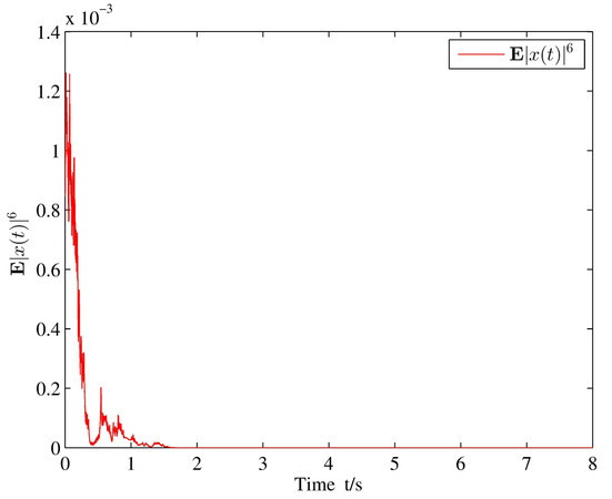
Figure 2. The exponential stability in $$ L^6 $$ of system (30).

Stability analysis for highly nonlinear switched stochastic systems with time-varying delays

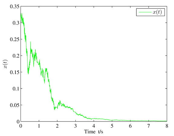
Figure 3. Exponential stability in the sample path of the system (30).

Stability analysis for highly nonlinear switched stochastic systems with time-varying delays

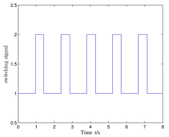
Figure 4. Switching signal $$ \sigma(t) $$ .

5. CONCLUSIONS

In this paper, the existence of a unique global solution for a highly nonlinear SSS with a deterministic switching signal is examined by using the ADT method coupled with the MLF approach. The stability criteria of $$ q $$ th moment exponential stability and almost surely exponential stability of the highly nonlinear SSS are stated. Finally, a numerical example is presented to illustrate the effectiveness of the obtained results. Inspired by recent studies [7, 20, 33-36], two further research directions have emerged: (1) Solving the problem of stability for highly nonlinear SSSs with impulsive effects under asynchronous switching, and (2) designing a control input function to stabilize a highly nonlinear SSS with a time-varying delay.

DECLARATIONS

Authors' contributions

Made substantial contributions to supervision, writing, review, editing and methodology: Wang H

Performed writing-original draft, software, validation and visualization: Sun J

Availability of data and materials

Not applicable.

Financial support and sponsorship

This work was jointly supported by the National Natural Science Foundation of China (62003170), and the Natural Science Foundation of Jiangsu Province (BK20190770).

Conflicts of interest

All authors declared there are no conflicts of interest.

Ethical approval and consent to participate

Not applicable.

Consent for publication

Not applicable.

Copyright

© The Author(s) 2022.

REFERENCES

1. Zhang R, Quan Q, Cai KY. Attitude control of a quadrotor aircraft subject to a class of time-varying disturbances. IET Control Theory & Applications 2011;5:1140-6.

2. Yoshida T, Jones LE, Ellner SP, Fussmann GF, Hairston NG Jr. Rapid evolution drives ecological dynamics in a predator-prey system. Nature 2003;424:303-6.

3. Preis T, Schneider JJ, Stanley HE. Switching processes in financial markets. Proc Natl Acad Sci U S A 2011;108:7674-8.

4. Mao XR, Yuan CG. Stochastic Differential Equations with Markovian Switching. London: Imperial College Press, 2006.

5. Wu XT, Tang Y, Cao JD. Input-to-state stability of time-varying switched systems with time delay. IEEE Trans Automat Contr 2019;64:2537-44.

6. Xiao HN, Zhu QX, Karimi HR. Stability of stochastic delay switched neural networks with all unstable subsystems: a multiple discretized Lyapunov-Krasovskii functionals method. Inf Sci 2022;582:302-15.

7. Yuan S, Zhang LX, Schutter BD, Baldi S. A novel Lyapunov function for a non-weighted $$ \mathcal{L}_2$$ gain of asynchronously switched linear systems. Automatica 2018;87:310-17.

8. Cheng P, He SP, Luan XL, Liu F. Finite-region asynchronous $H_{\infty}$$ control for 2D Markov jump systems. Automatica 2021;129:109590.

9. Wang B, Zhu QX. Stability analysis of Markov switched stochastic differential equations with both stable and unstable subsystems. Systems & Control Letters 2017;105:55-61.

10. Liberzon D. Finite data-rate feedback stabilization of switched and hybrid inear systems. Automatica 2014;50:409.

11. https://doi.org/10.1007/978-0-85729-256-8 [Last accessed on 22 Dec 2022] ]]>.

12. Hu LJ, Mao XR, Shen Y. Stability and boundedness of nonlinear hybrid stochastic differential delay equations. Syst & Contr Let 2013;62:178.

13. Li XY, Mao XR. Stabilisation of highly nonlinear hybrid stochastic differential delay equations by delay feedback control. Automatica 2020;112:108657.

14. Zhu QX. Stabilization of stochastic nonlinear delay systems with exogenous disturbances and the event-triggered feedback control. IEEE Trans Automat Contr 2019;64:3764-71.

15. Zhu QX, Song SY, Shi P. Effect of noise on the solutions of non-linear delay systems. IET Control Theory & Appl 2018;12:1822-9.

16. Dong HL, Mao XR. Advances in stabilization of highly nonlinear hybrid delay systems. Automatica 2022;136:110086.

17. Zhao Y, Wu XT, Gao JD. Stability of highly non-linear switched stochastic systems. IET Control Theory & Applications 2019;13:1940-44.

18. Liu L, Yin S, Zhang LX, Yin XY, Yan HC. Improved results on asymptotic stabilization for stochastic nonlinear time-delay systems with application to a chemical reactor system. IEEE Transactions on Sysems, Man, and Cybernetics: Systems 2016;47:195-204.

19. Hu W, Zhu QX, Karimi HR. Some improved razumikhin stability criteria for impulsive stochastic delay differential systems. IEEE Trans Automat Contr 2019;64:5207-13.

20. Yuan S, Zhang LX, Baldi S. Adaptive stabilization of impulsive switched linear time-delay systems: a piecewise dynamic gain approach. Automatica 2019;103:322-29.

21. Lian J, Feng Z. Passivity analysis and synthesis for a class of discrete-time switched stochastic systems with time-varying delay. Asian J Control 2013;15:501-11.

22. Cong S, Yin LP. Exponential stability conditions for switched linear stochastic systems with time-varying delay. IET Control Theory & Applications 2012;6:2453-59.

23. Yue D, Han QL. Delay-dependent exponential stability of stochastic systems with time-varying delay, nonlinearity, and markovian switching. IEEE Trans Automat Contr 2005;50:217-22.

24. Zeng HB, Liu XG, Wang W. A generalized free-matrix-based integral inequality for stability analysis of time-varying delay systems. Applied Mathematics and Computation 2019;354:1-8.

25. Chen HB, Shi P, Lim CC, Hu P. Exponential stability for neutral stochastic markov systems with time-varying delay and its applications. IEEE Trans Cybernetics 2015;46:1350-62.

26. Mao XR. Stochastic differential equations and applications. Elsevier; 2007.

27. Zhao Y, Zhu QX. Stability of highly nonlinear neutral stochastic delay systems with non-random switching signals. Syst & Contr Let 2022;165:105261.

28. Zhao Y, Zhu QX. Stabilization by delay feedback control for highly nonlinear switched stochastic systems with time delays. Int J Robust Nonlinear Control 2021;31:3070-89.

29. Fei WY, Hu LJ, Mao XR, Shen MX. Structured robust stability and boundedness of nonlinear hybrid delay systems. SIAM J Control Optim 2018;56:2662-89.

30. Shen MX, Fei C, Fei WY, Mao XR. Stabilisation by delay feedback control for highly nonlinear neutral stochastic differential equations. Syst & Contr Let 2020;137:104645.

31. Shen MX, Fei WY, Mao XR, Deng SN. Exponential stability of highly nonlinear neutral pantograph stochastic differential equations. Asian J Control 2020;22:436-48.

32. Song RL, Wang B, Zhu QX. Delay-dependent stability of nonlinear hybrid neutral stochastic differential equations with multiple delays. Int J Robust Nonlinear Control 2021;31:250-67.

33. Kang Y, Zhai DH, Liu GP, Zhao YB, Zhao P. Stability analysis of a class of hybrid stochastic retarded systems under asynchronous switching. IEEE Trans on Automat Contr 2014;59:1511-23.

34. Shen MX, Fei C, Fei WY, Mao XR, Mei CH. Delay-dependent stability of highly nonlinear neutral stochastic functional differential equations. Intl J Robust & Nonlinear 2022;32:9957-76.

35. Ren MF, Zhang QC, Zhang JH. An introductory survey of probability density function control. Syst Sci & Contr Eng 2019;7:158-70.

36. Zhang QC, Wang H. A novel data-based stochastic distribution control for non-Gaussian stochastic systems. IEEE Trans Automat Contr 2021;67:1506-13.

Cite This Article

Export citation file: BibTeX | RIS

OAE Style

Sun J, Wang H. Stability analysis for highly nonlinear switched stochastic systems with time-varying delays. Complex Eng Syst 2022;2:17. http://dx.doi.org/10.20517/ces.2022.48

AMA Style

Sun J, Wang H. Stability analysis for highly nonlinear switched stochastic systems with time-varying delays. Complex Engineering Systems. 2022; 2(4): 17. http://dx.doi.org/10.20517/ces.2022.48

Chicago/Turabian Style

Sun, Jing, Hui Wang. 2022. "Stability analysis for highly nonlinear switched stochastic systems with time-varying delays" Complex Engineering Systems. 2, no.4: 17. http://dx.doi.org/10.20517/ces.2022.48

ACS Style

Sun, J.; Wang H. Stability analysis for highly nonlinear switched stochastic systems with time-varying delays. Complex. Eng. Syst. 2022, 2, 17. http://dx.doi.org/10.20517/ces.2022.48

About This Article

Special Issue

© The Author(s) 2022. Open Access This article is licensed under a Creative Commons Attribution 4.0 International License (https://creativecommons.org/licenses/by/4.0/), which permits unrestricted use, sharing, adaptation, distribution and reproduction in any medium or format, for any purpose, even commercially, as long as you give appropriate credit to the original author(s) and the source, provide a link to the Creative Commons license, and indicate if changes were made.

Data & Comments

Data

Views
1288
Downloads
741
Citations
1
Comments
0
9

Comments

Comments must be written in English. Spam, offensive content, impersonation, and private information will not be permitted. If any comment is reported and identified as inappropriate content by OAE staff, the comment will be removed without notice. If you have any queries or need any help, please contact us at support@oaepublish.com.

0
Download PDF
Cite This Article 25 clicks
Like This Article 9 likes
Share This Article
Scan the QR code for reading!
See Updates
Contents
Figures
Related
Complex Engineering Systems
ISSN 2770-6249 (Online)

Portico

All published articles are preserved here permanently:

https://www.portico.org/publishers/oae/

Portico

All published articles are preserved here permanently:

https://www.portico.org/publishers/oae/