Faculty of Information Technology, Beijing University of Technology, Beijing 100124, China
Beijing Key Laboratory of Computational Intelligence and Intelligent System, Beijing University of Technology, Beijing 100124, China
Beijing Institute of Artificial Intelligence, Beijing University of Technology, Beijing 100124, China
Beijing Laboratory of Smart Environmental Protection, Beijing University of Technology, Beijing 100124, China
Correspondence to: Prof. Ding Wang, Faculty of Information Technology, Beijing University of Technology, 100 Pingleyuan,
Chaoyang District, Beijing 100124, China. E-mail: dingwang@bjut.edu.cn
Received: 17 Feb 2023 | First Decision: 6 Mar 2023 | Revised: 14 Mar 2023 | Accepted: 20 Mar 2023 | Published: 30 Mar 2023
Academic Editor: Yurong Liu | Copy Editor: Fanglin Lan | Production Editor: Fanglin Lan
Abstract
In this paper, the decentralized tracking control (DTC) problem is investigated for a class of continuous-time nonlinear systems with external disturbances. First, the DTC problem is resolved by converting it into the optimal tracking controller design for augmented tracking isolated subsystems (ATISs).
%It is investigated in the form of the nominal system. A cost function with a discount is taken into consideration. Then, in the case of external disturbances, the DTC scheme is effectively constructed via adding the appropriate feedback gain to each ATIS. %Herein, we aim to obtain the optimal control strategy for minimizing the cost function with discount. In addition, utilizing the approximation property of the neural network, the critic network is constructed to solve the Hamilton-Jacobi-Isaacs equation, which can derive the optimal tracking control law and the worst disturbance law. Moreover, the updating rule is improved during the process of weight learning, which removes the requirement for initial admission control. Finally, through the interconnected spring-mass-damper system, a simulation example is given to verify the availability of the DTC scheme.
For large-scale nonlinear interconnected systems, which are considered as nonlinear plants consisting of many interconnected subsystems, decentralized control has become a research hotspot in the last few decades [1–4]. Compared with the centralized control, the decentralized control has the advantages of simplifying the structure and reducing the computation burden of the controller. Besides, the local controller only depends on the information of the local subsystem. Meanwhile, with the development of science and technology, interconnected engineering applications have become increasingly complex, such as robotic systems [5] and power systems [6, 7]. In [8–10], we found that the decentralized control of the large-scale system was connected with the optimal control of the isolated subsystems, which means the optimal control method [11–14] can be adopted to achieve the design purpose of the decentralized controllers. However, the optimal control of the nonlinear system often needs to solve the Hamilton-Jacobi-Bellman (HJB) or Hamilton-Jacobi-Isaacs (HJI) equation, which can be solved by using the adaptive dynamic programming (ADP) method [15, 16]. Besides, in [13], Wang et al. investigated the latest intelligent critic framework for advanced optimal control. In [14], the optimal feedback stabilization problem was discussed with discounted guaranteed cost for nonlinear systems. It follows that the interconnection plays a significant role in designing the controller. Hence, it can be classified as decentralized and distributed control schemes. There is a certain distinction between decentralized control and distributed control. For decentralized control, each sub-controller only uses local information and the interconnection among subsystems can be assumed to be weak in nature. Compared with the decentralized control, the distributed control [17–19] can be introduced to improve the performance of the subsystems when the interconnections among subsystems become strong. In [20], the distributed optimal observer was devised to assess the nonlinear leader state for all followers. In [21], the distributed control was developed by means of online reinforcement learning for interconnected systems with exploration.
It is worth mentioning that the ADP algorithm has been extensively employed for dealing with various optimal regulation problems and tracking problems [22–24], which will achieve the goal, that is, the actual signal can track the reference signal under the noisy and the uncertain environment. In [25], Ha et al. proposed a novel cost function to explore the evaluation framework of the optimal tracking control problem. Then, aimed at complicated control systems, it is necessary to consider decentralized tracking control (DTC) problems [26–29]. The DTC systems can be transformed into the the nominal augmented tracking isolated subsystems (ATISs), which are composed of the tracking error and the reference signal. In [26], Qu et al. proposed a novel formulation consisting of a steady-state controller and a modified optimal feedback controller of the DTC strategy. Besides, the asymptotic DTC was realized by introducing two integral bounded functions in [27]. In [28], Liu et al. proposed a finite-time DTC method for a class of nonstrict feedback interconnected systems with disturbances. Moreover, the adaptive fuzzy output-feedback DTC design was investigated for switched large-scale systems in [29].
Game theory is a discipline that implements corresponding strategies. It contains cooperative and noncooperative types, that is, zero-sum (ZS) games and non-ZS games. In particular, ZS games have been widely applied in many fields [30–33]. The object of the ZS game is to derive the Nash equilibrium of nonliner systems, which makes the cost function optimized. In [31], the finite-horizon H-infinity state estimator design was studied for periodic neural networks over multiple fading channels. The noncooperative control problem was formulated as a two-player ZS game in [32]. In [33], Wang et al. investigated the stability of the general value iteration algorithm for ZS games. At the same time, we can also combine the ZS problem with the tracking problem to make the system more stable while achieving the trajectory tracking. In [34], Zhang et al. developed an online model-free integral reinforcement learning algorithm for solving the H-infinity optimal tracking problem for completely unknown systems. In [35], a general bounded $$ L_{2} $$ gain tracking policy was introduced with a discounted function. In [36], Hou et al. proposed an action-disturbance-critic neural network frame to realize the iterative dual heuristic programming algorithm.
As can be seen from the above, there are few studies that combine the DTC problem with the ZS game problem. It is necessary to take the related discounted cost function into account for the DTC system, which can transform the DTC problem into an optimal control problem with disturbances. In practice, the existence of disturbances will make an unpredictable impact on the plant. Hence, it is of vital importance to consider the stability of the DTC system. In the experimental simulation, it is a challenge to achieve the goal of effective online weight training, which is implemented under the tracking control law and the disturbance control law. Consequently, in this paper, we put forward a novel method in view of ADP to resolve the DTC problem with external disturbances for continuous-time (CT) nonlinear systems. More importantly, for the sake of overcoming the difficulty of selecting initial admissible control policies, an additional term is added during the weight updating process. Remarkably, in this paper, we introduce the discount factor for maximizing and minimizing the corresponding cost function.
The contributions of this paper are as follows: First, considering the disturbance input in the DTC system, the strategy feasibility and the system stability are discussed through theoretical proofs. It is worth noting that the discount factor is introduced to the cost function. Moreover, in the process of online weight training, we can make the DTC system reach a stable state without selecting the initial admissible control law. Additionally, we present the experimental process of the spring-mass-damper system. Besides, we derive the desired tracking error curves as well as control strategy curves, which demonstrates that they are uniformly ultimately bounded (UUB).
The whole paper is divided into six sections. The first section is the introduction of relevant background knowledges of the research content. The second section is the problem statement of basic problems about the two person ZS game and the DTC strategy. In the third section, we design the decentralized tracking controller by using the optimal control method through solving the HJI equations. Meanwhile, the relevant lemma and theorem are given to validate the establishment of the DTC strategy. In the fourth section, the design method in accordance with adaptive critic is elaborated. Most importantly, an improved critic learning rule is implemented via critic networks. In the fifth section, the practicability of this method is validated by an interconnected spring-mass-damper system. Finally, the sixth section displays conclusions and summarizes overall research content of the whole paper.
2. PROBLEM STATEMENT
Consider a CT nonlinear interconnected system with disturbances, which is composed of $$ N $$ interconnected subsystems. Its dynamic description can be expressed as
where $$ i={1, 2, \dotsc, N} $$, $$ x_{i}(t)\in{\mathbb R}^{n_{i}} $$ is the state vector of the $$ i $$th subsystem and $$ x(t) $$ denotes the partial interconnected state related to other subsystems of the large-scale system. $$ \bar{u}_{i} (x_{i}(t))\in{\mathbb R}^{m_{i}} $$ is the control input and $$ v_{i}(x_{i}(t))\in{\mathbb R}^{q_{i}} $$ is the external disturbance input. As for the $$ i $$th subsystem, we denote $$ f_{i}(x_{i}(t)) $$, $$ g_{i}(x_{i}(t)) $$, $$ h_{i}(x_{i}(t)) $$, and $$ \bar{Z}_{i}(x(t)) $$ as the nonlinear internal dynamics, the input gain matrix, the disturbance gain matrix, and the interconnected item in sequence. Besides, $$ {[{x}^{\mathit{T}}_{1}, {x}^{\mathit{T}}_{2}, \dotsc, {x}^{\mathit{T}}_{N}]}^{\mathit{T}}\in{\mathbb R}^{n} $$ denotes the whole state of the large-scale system Equation (1), where $$ n=\sum_{i=1}^{N}n_{i} $$. Accordingly, $$ {x_{1}, x_{2}, \dotsc, x_{N}} $$ are named local states and $$ \bar{u}_{1}(x_{1}), \bar{u}_{2}(x_{2}), \dotsc, \bar{u}_{N}(x_{N}) $$ are called local controllers. We let $$ R_{i}\in{\mathbb R}^{m_{i}\times m_{i}} $$ be the symmetric positive definite matrix and denote $$ Z_{i}(x(t))={R_{i}}^{{1}/{2}}\bar{Z}_{i}(x(t)) $$. In addition, $$ {Z}_{i}(x(t))\in{\mathbb R}^{m_{i}} $$ is bounded as follows:
where $$ j={1, 2, \dotsc, N} $$, $$ \alpha_{ij} $$ is the nonnegative constant, $$ \theta_{ij}(x_{j}) $$ is the positive semidefinite function. Besides, we define $$ \theta_{j}(x_{j})=\max{\{\theta_{1j}(x_{j}), \theta_{2j}(x_{j}), \dotsc, \theta_{Nj}(x_{j})\}} $$ and the element of $$ {\{\theta_{1j}(x_{j}), \theta_{2j}(x_{j}), \dotsc, \theta_{Nj}(x_{j})\}} $$ will not reach zero at the same time. For this reason, $$ \beta_{ij}\geq \alpha_{ij}\theta_{ij}(x_{j})/\theta_{j}(x_{j}) $$ holds, where $$ \beta_{ij} $$ is also the nonnegative constant.
In this paper, considering the nonlinear system Equation (1), a reference system is introduced as follows:
$$ \dot{r}_{i}(t)=\zeta_{i}(r_{i}(t)), $$
where $$ r_{i}(t)\in{\mathbb R}^{n_{i}} $$ denotes the desired trajectory with $$ r_{i}(0) = r_{i0} $$, the function $$ \zeta_{i} $$ is locally Lipschitz continuous satisfying $$ \zeta_{i}(0)=0 $$. For the $$ i $$th subsystem, the trajectory tracking error can be defined as $$ e_{i}(t)=x_{i}(t)-r_{i}(t) $$ with $$ e_{i}(0) = e_{i0} $$. Thus, the dynamics of the tracking error is
Noticing $$ x_{i}(t)=e_{i}(t)+r_{i}(t) $$, we define the augmented subsystem states as $$ y_{i}(t)=[{e}^{\mathit{T}}_{i}(t), {r}^{\mathit{T}}_{i}(t)]^{\mathit{T}}\in{\mathbb R}^{2n_{i}} $$ with $$ y_{i}(0)=y_{i0}=[{e}^{\mathit{T}}_{i0}, {r}^{\mathit{T}}_{i0}]^{\mathit{T}} $$. Hence, the dynamic of the $$ i $$th ATIS based on Equations (1) and (3) can be formulated as a concise form
where $$ \mathcal{F}_{i}(y_{i}(t))\in{\mathbb R}^{2n_{i}} $$, $$ \mathcal{G}_{i}(y_{i}(t))\in{\mathbb R}^{2n_{i}\times m_{i}} $$, and $$ \mathcal{H}_{i}(y_{i}(t))\in{\mathbb R}^{2n_{i}\times q_{i}} $$ respectively. Specifically, they can be expressed as
We aim to design a pair of decentralized control policies $$ \bar{u}_{1}, \bar{u}_{2}, \dotsc, \bar{u}_{N} $$ to ensure that large-scale system Equation (1) can track the desired object while being restricted by external disturbances. It means that as $$ t\to +\infty $$, $$ \|x_{i}(t)-r_{i}(t)\|\to 0 $$. Meanwhile, it is noteworthy that the control pair $$ \bar{u}_{1}, \bar{u}_{2}, \dotsc, \bar{u}_{N} $$ should be pointed out only as a corresponding controller with the local information. In what follows, it presents the DTC problem by transforming it into the optimal controller design of ATISs by considering an appropriate discounted cost function.
3. DTC DESIGN VIA OPTIMAL REGULATION
3.1. Optimal control and the HJI equations
In this section, the optimal DTC strategy of the ATIS with the disturbance rejection is elaborated. It is addressed by solving the HJI equation with a discounted cost function. Then, we consider the nominal part of the augmented system Equation (5) as
We assume that $$ \mathcal{F}_{i} +\mathcal{G}_{i}u_{i}+\mathcal{H}_{i}v_{i} $$ is Lipschitz continuous on a set $$ \Omega_{i}\subset{\mathbb R}^{2n_{i}} $$, which is commonly used in the field of adaptive critic control to ensure the existence and uniqueness of the solution for the differential equation. Related to the $$ i $$th ATIS, we manage to minimize and maximize the discounted cost function as
where $$ Q_{i}\in{\mathbb R}^{2n_{i}\times2n_{i}} $$, $$ R_{i}\in{\mathbb R}^{m_{i}\times m_{i}} $$ are both positive definite matrices. Herein, we let $$ {y}^{\mathit{T}}_{i}Q_{i}y_{i}-{\varrho^2_{i}}{v}^{\mathit{T}}_{i}(y_{i})v_{i}(y_{i})=\gamma^{2}_{i}(y_{i}) $$ and $$ \theta_{i}(y_{i})\leq \sqrt{\gamma_{i}^{2}(y_{i})-\lambda_{i}J_{i}(y_{i})} $$, where $$ \gamma_{i}^{2}(y_{i})>\lambda_{i}J_{i}(y_{i}) $$. It is worth noting that this inequality is employed to prove the feasibility of Theorem 1. Then, Equation (10) can be equivalent to
If Equation (11) is continuously differentiable, the nonlinear Lyapunov equation is the infinitely small form of Equation (11). The Lyapunov equation is as follows:
Due to the saddle point solution $$\{ u_{i}^* $$, $$ v_{i}^* \}$$ satisfies the extremum theorem, the optimal tracking control law and the worst disturbance law can be computed by
In the following, we present the DTC strategy by adding the feedback gain to the interconnected system Equation (5). Herein, the following lemma is given by
Lemma 1 Considering the ATIS Equation (9), the feedback control
$$ \bar{u}_{i}(y_{i})=k_{i}u_{i}^*(y_{i}) $$
can ensure the $$ N $$ ATISs are asymptotically stable as long as $$ k_{i}\geq1/2 $$, which makes the tracking error approach to zero.
Proof. The lemma can be proved by showing $$ J_{i}^*(y_{i}) $$ is a candidate Lyapunov function. We can find $$ J_{i}^*(y_{i})\ge0 $$ in Equation (11), which implies that $$ J_{i}^*(y_{i}) $$ is a positive definite function. The derivative of $$ J_{i}^*(y_{i}) $$ along with the $$ i $$th ATIS is given by
Observing Equation (21), we can obtain that $$ \dot{J}_{i}^*(y_{i})<0 $$ holds under the condition $$ \gamma^{2}_{i}(y_{i})>\lambda_{i}J_{i}^*(y_{i}) $$ for all $$ k_{i}\geq1/2 $$ and $$ y_{i}\neq0 $$. Thus, the conditions are satisfied for Lyapunov local stability theory and the actual state of each ATIS can realize desired tracking objectives under the feedback control strategy. The proof is completed.
Remark 1.It is worth mentioning that only when $$ k_{i}= 1 $$, the feedback control is optimal. Then, we will show the following theorem to verify the proposed control law can effectively establish the DTC strategy.
Theorem 1 Taking Equation (2) and the interconnected augmented tracking system Equation (5) into account, there exist $$ N $$ positive numbers $$ {k}_{i}^* $$, such that, for any $$ {k}_{i}>{k}_{i}^* $$, the feedback control polices given by Equation (19) guarantee that the interconnected tracking system can maintain the asymptotic stability. In other words, the control pair $$ \bar{u}_{1}(y_{1}), \bar{u}_{2}(y_{2}), \dotsc, \bar{u}_{N}(y_{N}) $$ is the DTC strategy for the large-scale system.
Proof. Inspired by Lemma 1, we observe that $$ J_{i}^*(y_{i}) $$ is the Lyapunov function. Therefore, a composite Lyapunov function of $$ {J}_{i}^*(y_{i}) $$ is chosen as
Considering Equation (2), the mentioned inequality $$ \theta_{i}(y_{i})\leq \sqrt{\gamma_{i}^{2}(y_{i})-\lambda_{i}J_{i}(y_{i})} $$, where $$ \gamma_{i}^{2}(y_{i})>\lambda_{i}J_{i}(y_{i}) $$, and Equation (21), the upper formula can be converted to
Therefore, we introduce a 2$$ N $$-dimensional column vector $$ \vartheta $$, which consists of the $$ N $$-dimensional column vector $$ \sqrt{\gamma_{i}^{2}(y_{i})-\lambda_{i}J_{i}(y_{i})} $$ and the $$ N $$-dimensional column vector $$ \left\|{(\nabla J_{i}^*(y_{i}))}^{\mathit{T}}\mathcal{G}_{i}(y_{i})R_{i}^{-\frac{1}{2}}\right\| $$. Its form is as follows:
According to Equation (29), it can be concluded that when $$ k_{i} $$ is sufficiently large, the matrix $$ \mathscr{A} $$ is positive definite, which means there exist $$ {k}_{i}^* $$ so that any $$ {k}_{i}>{k}_{i}^* $$ sufficiently large to ensure the positive definite property of $$ \mathscr{A} $$. Then, we get $$ \dot{\mathcal{L}}(y)<0 $$. Consequently, the DTC strategy with external disturbances is constructed. The proof is completed.
Obviously, the key point of designing the DTC strategy is to obtain the optimal controller of the ATIS based on Theorem 1. Next, for the sake of getting hold of optimal controllers for the $$ N $$ ATISs by solving the HJI equations, in the following, we employ the ADP method to obtain the approximate optimal solutions by means of critic networks.
4. OPTIMAL DTC DESIGN VIA NEURAL NETWORKS
4.1. Implementation procedure via neural networks
In this section, we show the process of finding the approximate optimal solution by employing the ADP method based on neural networks. The critic networks have the capability of approximating nonlinear mapping, and the approximate cost function can be derived for the DTC system. Hence, $$ J_{i}^*(y_{i}) $$ can be expressed as
where $$ w_{ci}\in{\mathbb R}^{l_{ci}} $$ is the ideal weight vector, $$ l_{ci} $$ is the number of neurons in the hidden layer, $$ \sigma_{ci}(y_{i})\in{\mathbb R}^{l_{ci}} $$ is the activation function, and $$ \xi_{ci}(y_{i}) $$ is the reconstruction error of the $$ i $$th neural network. The gradient of $$ J_{i}^*(y_{i}) $$ is formulated as
where $$ e_{chi} $$ is the residual error of the neural network. To avoid the unknown ideal weight vector, we construct $$ N $$ critic neural networks to approximate $$ J_{i}^*(y_{i}) $$ as
where $$ \tilde{w}_{ci}=w_{ci}-\hat{w}_{ci} $$ is the weight error vector. At present, in order to minimize the objective function $$ E_{ci}=({1}/{2})e^{\mathit{T}}_{ci}e_{ci} $$, the normalised steepest descent algorithm based on Equation (38) is employed as follows:
where $$ \eta_{ci}>0 $$ represents the basic learning rate. Besides, $$ (1+\phi^{\mathit{T}}_{i}\phi_{i})^2 $$ is introduced for the normalization to simplify the critic error dynamics, and $$ \phi_{i} $$ is derived as
Usually, in the traditional weight training process, it is often necessary to select the appropriate initial weight vector for effective training. To eliminate the initial admissible control law, an improved critic learning rule is presented in the following.
4.2. Improved critic learning rule via neural networks
Herein, an additional Lyapunov function is introduced for the purpose of improving the critic learning mechanism. Then, the following rational assumption is given.
Assumption 1 Consider the dynamic of the $$ i $$th ATIS Equation (9) with the optimal cost function Equation (14) and the closed-loop optimal control policy Equation (32). We select $$ J_{si}(y_{i}) $$ as a continuously differentiable Lyapunov function and have the following relation:
where $$ s_{mi} $$ is the minimum eigenvalue of the matrix $$ \mathscr{B} $$.
Remark 2.Herein, the motivation of selecting the cost function $$ J_{si}(y_{i}) $$ is to obtain the optimal DTC strategy, which can minimize and maximize $$ J_{si}(y_{i}) $$ under the optimal control law and the worst disturbance law. Moreover, we can discuss the stability of closed-loop systems by the constructed optimal cost function. Besides, just to be clear, $$ J_{si}(y_{i}) $$ is derived by properly selecting the quadratic polynomial in terms of the state vector. We generally choose $$ J_{si}(y_{i})=0.5{y_{i}}^{\mathit{T}}y_{i} $$.
When the condition occurs, that is, $$ (\nabla J_{si}(y_{i}))^{\mathit{T}}[\mathcal{F}_{i}(y_{i})+\mathcal{G}_{i}(y_{i}){u}_{i}^*(y_{i}) +\mathcal{H}_{i}(y_{i})v_{i}^*(y_{i})] $$$$ >0 $$, which means the system is in an unstable state under the optimal control law Equation (36). In this case, an additional term is introduced to ensure the system stability. Based on Equation (36), some processing is performed as follows:
where $$ \eta_{si}>0 $$ represents the additional learning rate with respect to the stabilising term and $$ \Pi_{i}(y_{i}, \hat{u}_{i}^*, \hat{v}_{i}^*) $$ stands for the adaptation parameter term that tests the stability of the ATIS. The definition of $$ \Pi_{i} $$ is as follows:
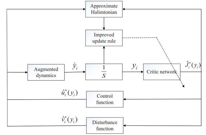
It is found that when the derivative of $$ J_{si}(y_{i}) $$ satisfies $$ \dot{J}_{si}(y_{i})<0 $$, the latter term of the weight update rule does not play its role so that the update mode is still the traditional normalized steepest descent algorithm. When $$ \dot{J}_{si}(y_{i})>0 $$, the latter term of the weight update rule starts to play its role of ensuring the stability, that is, the improved weight update method is adopted. It can be seen that the system can be adjusted to be stable under the improved weight updating criterion. Moreover, in order to clearly highlight that we have achieved the elimination of the initial admissible control law, herein, we set the initial weight vector to zero. Through the new critic learning rule, the structure of the proposed DTC strategy for ATIS is performed in Figure 1.
Figure 1. Control structure of the ATIS. ATIS: augmented tracking isolated subsystem。
In accordance to $$ \dot{\tilde{w}}_{ci}=-\dot{\hat{w}}_{ci} $$ and Equation (39), the specific form of $$ {\tilde{w}}_{ci} $$ is derived. Then, we can convert the estimated weight $$ \hat{w}_{ci} $$ into the form of the weight vector $$ {w}_{ci} $$ and the error weight vector $$ \tilde{w}_{ci} $$, which can be employed by proving the state $$ y_{i} $$ and the weight estimation error $$ \tilde{w}_{ci} $$ are UUB for the closed-loop system.
5. SIMULATION EXPERIMENT
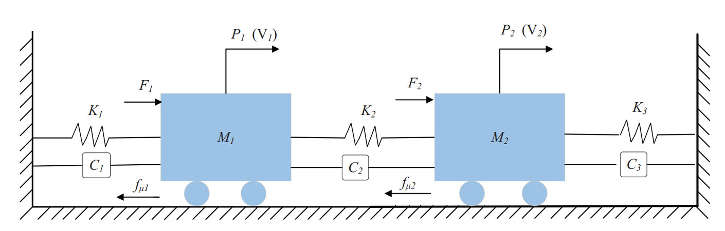
In this section, we will introduce the common mechanical vibration system, that is, the spring-mass-damper system. The structural diagram of the mechanical system is shown in Figure 2. From it, $$ M_{1} $$ and $$ M_{2} $$ denote the mass of two objects, $$ K_{1} $$, $$ K_{2} $$, and $$ K_{3} $$ represent the stiffness constants of three springs. $$ C_{1} $$, $$ C_{2} $$, and $$ C_{3} $$ stand for the damping, respectively.
Figure 2. Simple diagram of the interconnected mass–spring–damper system.
In addition, let $$ P_{i} $$, $$ V_{i} $$, $$ F_{i} $$, and $$ f_{\mu_{i}} $$ be the position, the velocity, the force, and the friction applied to the object, where $$ i=1, 2 $$. Hence, the system dynamics for $$ M_{1} $$ and $$ M_{2} $$ are as follows:
For the object $$ M_{1} $$, we define $$ x_{11}=P_{1} $$, $$ x_{12}=V_{1} $$, $$ \bar{u}_{1}(x_{1})=F_{1} $$, and $$ {v}_{1}(x_{1})=f_{\mu_{1}} $$. In the same way, we let $$ x_{21}=P_{2} $$, $$ x_{22}=V_{2} $$, $$ \bar{u}_{2}(x_{2})=F_{2} $$, and $$ {v}_{2}(x_{2})=f_{\mu_{2}} $$ for the object $$ M_{2} $$. Next, the state-space of the spring-mass-damper system is written as
where $$ x_{1}=[x_{11}, x_{12}]^{\mathit{T}}\in{\mathbb R}^{2} $$ and $$ x_{2}=[x_{21}, x_{22}]^{\mathit{T}}\in{\mathbb R}^{2} $$ are system states. $$ \bar{u}_{1}(x_{1})\in{\mathbb R} $$, $$ \bar{u}_{2}(x_{2})\in{\mathbb R} $$, $$ v_{1}(x_{1})\in{\mathbb R} $$, and $$ v_{2}(x_{2})\in{\mathbb R} $$ are control inputs and disturbance inputs of the subsystem 1 and the subsystem 2, respectively. Simultaneously, $$ Z_{1}(x)=K_{2}\left(x_{21}-x_{11}\right)+C_{2}\left(x_{22}-x_{12}\right) $$ and $$ Z_{2}(x)=K_{2}\left(x_{11}-x_{21}\right)+C_{2}\left(x_{12}-x_{22}\right) $$, which indicates the spring $$ K_{2} $$ and the damping $$ C_{2} $$ play a connecting role for two subsystems. Herein, we let $$ \theta_{1}(x_{1})= ||x_{1}|| $$ and $$ \theta_{2}(x_{2})= |x_{22}| $$. Besides, we choose $$ \beta_{11}=\beta_{12}=1 $$, $$ \beta_{21}=\beta_{22}=1/2 $$, and $$ {\mu_{1}}={\mu_{2}}=1 $$. Moreover, we select $$ \lambda_{1}=\lambda_{2}=0.6 $$, $$ \varrho_{1}=\varrho_{2}=1 $$, $$ R_{1}=R_{2}=2 $$, and $$ Q_{1}=Q_{2}=2I_{4} $$, where $$ I_{4} $$ is the four-dimensional identity matrix. Above all, the desired reference trajectories $$ r_{1} $$ and $$ r_{2} $$ for two subsystems are generated by the following command system:
where $$ r_{1}=[r_{11}, r_{12}]^{\mathit{T}}\in{\mathbb R}^{2} $$ and $$ r_{2}=[r_{21}, r_{22}]^{\mathit{T}}\in{\mathbb R}^{2} $$ are reference states. Then, we define the tracking errors as $$ e_{i1}=x_{i1}-r_{i1} $$ and $$ e_{i2}=x_{i2}-r_{i2} $$. Hence, the augmented state vector can be expressed as $$ y_{i}=[y_{i1}, y_{i2}, y_{i3}, y_{i4}]^{\mathit{T}}=[e_{i1}, e_{i2}, r_{i1}, r_{i2}]^{\mathit{T}} $$, $$ i=1, 2 $$. We set practical parameters as $$ M_{1}=1 $$kg, $$ K_{1}=3 $$N/m, and $$ C_{1}=0.5 $$Ns/m for the subsystem 1. Similarly, we let $$ M_{2}=2 $$kg, $$ K_{3}=5 $$N/m, and $$ C_{3}=1 $$Ns/m for the subsystem 2. Considering Equations (51-53), the augmented system dynamics $$ \dot{y}_{1} $$ and $$ \dot{y}_{2} $$ can be obtained in the following forms:
During the online learning process, we take basic learning rates and additional learning rates as $$ \eta_{c1}=0.01 $$, $$ \eta_{c2}=0.03 $$ as well as $$ \eta_{s1}=\eta_{s2}=0.01 $$. Let initial system states and reference states be $$ x_{10}=[1.5, 0]^{\mathit{T}} $$, $$ x_{20}=[1, -1]^{\mathit{T}} $$, and $$ r_{10}=r_{20}=[0.5, -0.5]^{\mathit{T}} $$, respectively. Therefore, initial states of the ATIS are $$ y_{10}=[1, 0.5, 0.5, -0.5]^{\mathit{T}} $$ and $$ y_{20}=[0.5, -0.5, 0.5, -0.5]^{\mathit{T}} $$.
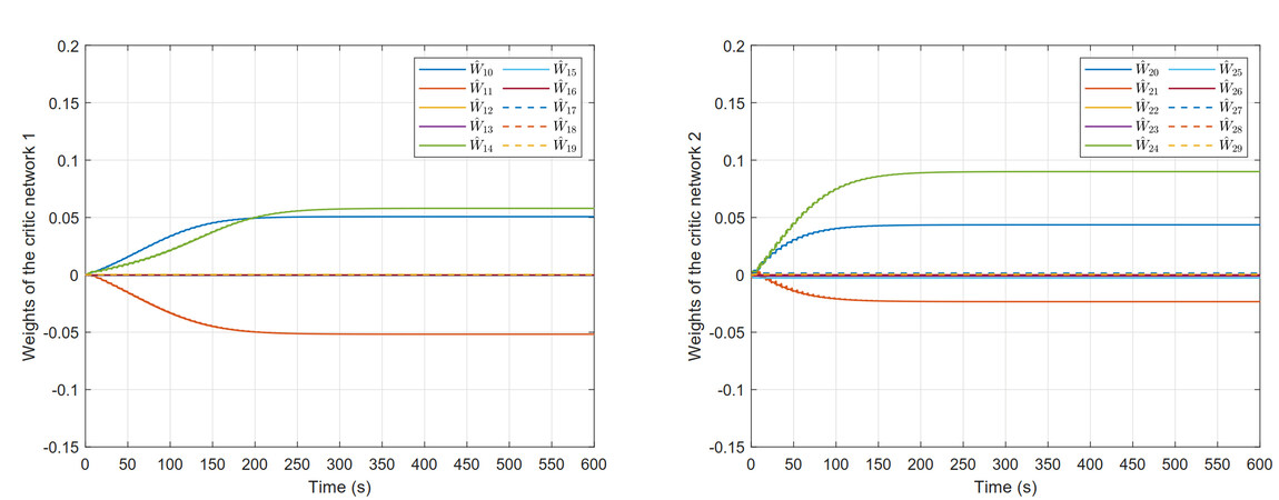
Herein, two probing noises are added within the beginning 400 steps to keep the persistence of excitation condition of the ATIS. The weight convergence curves are shown in Figure 3. It can be seen that the weight has converged to a certain numerical value before turning off the excitation condition, which confirms the validity of the improved weight update algorithm. Form it, we find the initial weights are selected as zero, which indicates the initial admissible control is eliminated.
Figure 3. Weights convergence process of the critic network 1 and the critic network 2.
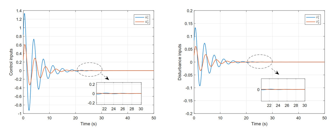
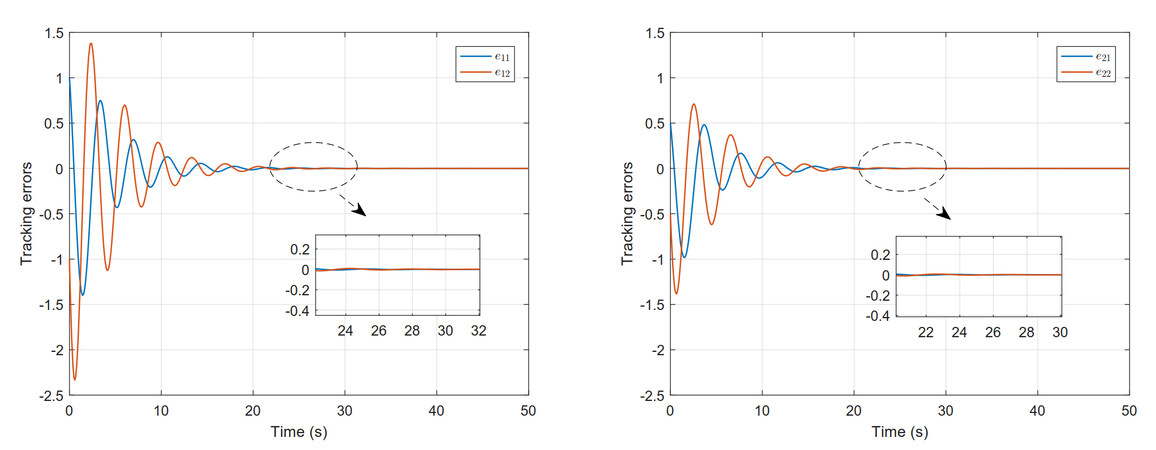
Next, in order to make the system achieve the purpose of the optimal tracking, feedback gains are selected as $$ k_{1}=k_{2}=1 $$. Then, the DTC strategy $$ \{k_{1}\hat u_{1}^*(y_{1}), k_{2}\hat u_{2}^*(y_{2}) \}$$ can be derived from the obtained weight vector for the spring-mass-damper interconnected system. In addition, the evolution curves are shown in Figure 4, which displays the tracking control inputs and disturbance inputs for the subsystem 1 and the subsystem 2. Then, the obtained DTC strategy is applied to the controlled system for 50 s, and its tracking error trajectory curves are displayed in Figure 5. It is obvious that the tracking error curves are eventually enforced to the origin. Taken together, this simulation result verifies the effectiveness of the proposed DTC strategy.
Figure 4. Tracking control inputs and disturbance inputs for subsystem 1 and subsystem 2.
Figure 5. Tracking error trajectories for subsystem 1 and subsystem 2.
6. CONCLUSION
In this paper, the optimal DTC strategy for CT nonlinear large-scale systems with external disturbances is proposed by employing the ADP algorithm. The approximate optimal control law of the ATISs can achieve the trajectory tracking goal. Then, the establishment of the DTC strategy is derived by adding the appropriate feedback gain, whose feasibility has been proved via the Lyapunov theory. Note that all the above-mentioned results are investigated by considering a cost function with the discount. Then, only a series of single critic networks are employed to solve HJI equations of $$ N $$ ATISs, so that we acquire the approximate optimal control law and the worst disturbance law. In addition, the stability term added in the weight updating process avoids the selection of the initial stable control policy. Furthermore, the simulation results are displayed for the spring-mass-damper system to indicate the validity of the proposed DTC method. In the future, we will utilize more advanced methods to deal with the DTC problem for nonaffine systems. Besides, we can also consider the unmatched interconnected relationship for the DTC problem, which is a considerable direction of improved research.
DECLARATIONS
Authors' contributions
Made significant contributions to the conception and experiments: Fan W, Wang D
Made significant contributions to the writing: Fan W, Wang D
Made substantial contributions to the revision and translation: Liu A, Wang D
Availability of data and materials
Not applicable
Financial support and sponsorship
This work was supported in part by the National Natural Science Foundation of China (No. 62222301; No. 61890930-5 and No. 62021003); in part by the National Key Research and Development Program of China (No. 2021ZD0112302; No. 2021ZD0112301 and No. 2018YFC1900800-5); and in part by the Beijing Natural Science Foundation (No. JQ19013).
Conflicts of interest
All authors declared that there are no conflicts of interest.
1. Saberi A. On optimality of decentralized control for a class of nonlinear interconnected systems. Automatica 1988;24:1101-4.
2. Mu CX, Sun CY, Wang D, Song AG, Qian CS. Decentralized adaptive optimal stabilization of nonlinear systems with matched interconnections. Soft Comput 2018;22:82705-15.
3. Mehraeen S, Jagannathan S. Decentralized optimal control of a class of interconnected nonlinear discrete-time systems by using online Hamilton-Jacobi-Bellman formulation. IEEE Trans Neural Netw 2011;22:111715-96.
4. Yang X, He HB. Adaptive dynamic programming for decentralized stabilization of uncertain nonlinear large-scale systems with mismatched interconnections. IEEE Trans Syst Man Cybern Syst 2020;50:82870-82.
5. Karimi HR. How to deal with the complexity in robotic systems? Complex Eng Syst 2022;2:15.
6. Xu Q, Yu C, Yuan X, Fu Z, Liu H. A distributed electricity energy trading strategy under energy shortage environment. Complex Eng Syst 2022;2:14.
7. Bian T, Jiang Y, Jiang ZP. Decentralized adaptive optimal control of large-scale systems with application to power systems. IEEE Trans, Ind Electron 2015;62:42439-47.
8. Liu DR, Wang D, Li HL. Decentralized stabilization for a class of continuous-time nonlinear interconnected systems using online learning optimal control approach. IEEE Trans Neural Netw Learn Syst 2014;25:2418-28.
9. Sun KK, Sui S, Tong SC. Fuzzy adaptive decentralized optimal control for strict feedback nonlinear large-scale systems. IEEE Trans, Cybern 2018;48:41326-39.
10. Wang XM, Feng ZG, Zhang GJ, Niu B, Yang D, et al. Adaptive decentralised control for large-scale non-linear non-strict-feedback interconnected systems with time-varying asymmetric output constraints and dead-zone inputs. IET Control Theory & Appl 2020;14:203417-27.
11. Wei QL, Liu DR, Lin Q, Song RZ. Discrete-time optimal control via local policy iteration adaptive dynamic programming. IEEE Trans, Cybern 2017;47:103367-79.
12. Wang D, Ren J, Ha MM, Qiao JF. System stability of learning-based linear optimal control with general discounted value iteration. IEEE, Trans Neural Netw Learn Syst 2022:Online ahead of print.
13. Wang D, Ha MM, Zhao MM. The intelligent critic framework for advanced optimal control. Artif Intell Rev 2022;55:11-22.
14. Wang D, Qiao JF, Cheng L. An approximate neuro-optimal solution of discounted guaranteed cost control design. IEEE Trans Cybern 2022;52:177-86.
15. Li YM, Liu YJ, Tong SC. Observer-based neuro-adaptive optimized control of strict-feedback nonlinear systems with state constraints. IEEE Trans Neural Netw Learn Syst 2022;33:73131-45.
16. Wang H, Yang CY, Liu XM, Zhou LN. Neural-network-based adaptive control of uncertain MIMO singularly perturbed systems with full-state constraints. IEEE Trans Neural Netw Learn Syst 2021; doi: 10.1109/TNNLS.2021.3123361.
17. Zhang H, Hong QQ, Yan HC, Yang FW, Guo G. Event-based distributed H-infinity filtering networks of 2-DOF quarter-car suspension systems. IEEE Trans Ind Inform 2017;13:1312-21.
18. Chen YG, Fei SM, Li YM. Robust stabilization for uncertain saturated time-delay systems: A distributed-delay-dependent polytopic approach. IEEE Trans Automat Contr 2017;62:73455-60.
19. Chen YG, Wang ZD. Local stabilization for discrete-time systems with distributed state delay and fast-varying input delay under actuator saturations. IEEE Trans Automat Contr 2021;66:31337-44.
20. Fu H, Chen X, Wu M. Distributed optimal observer design of networked systems via adaptive critic design. IEEE Trans Syst Man Cybern, Syst 2021;51:116976-85.
21. Narayanan V, Jagannathan S. Event-triggered distributed control of nonlinear interconnected systems using online reinforcement learning with exploration. IEEE Trans Cybern 2018;48:92510-9.
22. Wang D, Zhao MM, Ha MM, Qiao JF. Intelligent optimal tracking with application verifications via discounted generalized value iteration. Acta Automatica Sinica 2022;48:1182-93.
23. Zhang HG, Zhang K, Cai YL, Han J. Adaptive fuzzy fault-tolerant tracking control for partially unknown systems with actuator faults via integral reinforcement learning method. IEEE Trans Fuzzy Syst 2019;27:101986-98.
24. Modares H, Lewis FL. Optimal tracking control of nonlinear partially-unknown constrained-input systems using integral reinforcement learning. Automatica 2014;50:71780-1792.
25. Ha MM, Wang D, Liu DR. Discounted iterative adaptive critic designs with novel stability analysis for tracking control. IEEE/CAA, Journal of Automat Sinica 2022;9:71262-1272.
26. Qu QX, Zhang HG, Feng T, Jiang H. Decentralized adaptive tracking control scheme for nonlinear large-scale interconnected systems via adaptive dynamic programming. Neurocomputing 2017;225:1-10.
27. Niu B, Liu JD, Wang D, Zhao XD, Wang HQ. Adaptive decentralized asymptotic tracking control for large-scale nonlinear systems with unknown strong interconnections. IEEE/CAA Journal of Automatica Sinica 2022;9:1173-86.
28. Liu JD, Niu B, Kao YG, Zhao P, Yang D. Decentralized adaptive command filtered neural tracking control of large-scale nonlinear systems: An almost fast finite-time framework. IEEE Trans Neural Netw Learn Syst 2021;32:83621-2.
29. Tong SC, Zhang LL, Li YM. Observed-based adaptive fuzzy decentralized tracking control for switched uncertain nonlinear large-scale systems with dead zones. IEEE Trans Syst Man Cybern Syst 2016;46:137-47.
30. Wang D, Hu LZ, Zhao MM, Qiao JF. Dual event-triggered constrained control through adaptive critic for discrete-time zero-sum games. IEEE Trans Syst Man Cybern Syst 2023;53:31584-9.
31. Li XM, Zhang B, Li PS, Zhou Q, Lu RQ. Finite-horizon H-infinity state estimation for periodic neural networks over fading channels. IEEE Trans Neural Netw Learn Syst 2020;31:51450-60.
32. Duan JJ, Xu H, Liu WX, Peng JC, Jiang H. Zero-sum game based cooperative control for onboard pulsed power load accommodation. IEEE Trans Ind Inform 2020;16:1238-47.
33. Wang D, Zhao MM, Ha MM, Qiao JF. Stability and admissibility analysis for zero-sum games under general value iteration formulation. IEEE Trans Neural Netw Learn Syst 2022; doi: 10.1109/TNNLS.2022.3152268.
34. Zhang HG, Cui XH, Luo YH, Jiang H. Finite-horizon H-infinity tracking control for unknown nonlinear systems with saturating actuators. IEEE Trans Neural Netw Learn Syst 2018;29:41200-12.
35. Modares H, Lewis FL, Jiang ZP. H-infinity tracking control of completely unknown continuous-time systems via off-policy reinforcement learning. IEEE Trans Neural Netw Learn Syst 2015;26:102550-62.
36. Hou JX, Wang D, Liu DR, Zhang Y. Model-free H-infinity optimal tracking control of constrained nonlinear systems via an iterative adaptive learning algorithm. IEEE Trans Syst Man Cybern Syst 2020;50:114097-108.
Fan W, Liu A, Wang D. Decentralized tracking control design based on intelligent critic for an interconnected spring-mass-damper system. Complex Eng Syst 2023;3:5. http://dx.doi.org/10.20517/ces.2023.04
AMA Style
Fan W, Liu A, Wang D. Decentralized tracking control design based on intelligent critic for an interconnected spring-mass-damper system. Complex Engineering Systems. 2023; 3(1): 5. http://dx.doi.org/10.20517/ces.2023.04
Chicago/Turabian Style
Fan, Wenqian, Ao Liu, Ding Wang. 2023. "Decentralized tracking control design based on intelligent critic for an interconnected spring-mass-damper system" Complex Engineering Systems. 3, no.1: 5. http://dx.doi.org/10.20517/ces.2023.04
ACS Style
Fan, W.; Liu A.; Wang D. Decentralized tracking control design based on intelligent critic for an interconnected spring-mass-damper system. Complex. Eng. Syst.2023, 3, 5. http://dx.doi.org/10.20517/ces.2023.04
Comments must be written in English. Spam, offensive content, impersonation, and private information will not be permitted. If any
comment is reported and identified as inappropriate content by OAE staff, the comment will be removed without notice. If you have any
queries or need any help, please contact us at
support@oaepublish.com.

 0
0


 Cite This Article 31 clicks

 Like This Article 1
likes
Like This Article 1
likes


Comments
Comments must be written in English. Spam, offensive content, impersonation, and private information will not be permitted. If any comment is reported and identified as inappropriate content by OAE staff, the comment will be removed without notice. If you have any queries or need any help, please contact us at support@oaepublish.com.