Download PDF
Research Article  |  Open Access  |  19 May 2023

Nonlinear hierarchical control for four-wheel-independent-drive electric vehicle

Views: 738 |  Downloads: 247 |  Cited:   0
Complex Eng Syst 2023;3:8.
10.20517/ces.2022.50 |  © The Author(s) 2023.
Author Information
Article Notes
Cite This Article

Abstract

As under-constrained systems, four-wheel-independent-drive (4WID) electric vehicles have more driving degrees of freedom. In this context, reasonable control and distribution of driving or braking torque to each wheel is extremely important from the vehicle safety perspective. However, it is difficult to provide the optimal wheel torque because of the time-varying characteristics and typical over-actuated nature of the system. In light of these challenges, a novel hierarchical control scheme comprising a top- and bottom-level controller is proposed herein. First, for the top-level controller, a time-varying model-predictive-control (TV-MPC) controller is designed based on an extended 3-degree-of-freedom (3-DOF) reference vehicle model. The total driving force and additional yaw moment can be obtained using the TV-MPC. Second, for the bottom-level controller, the torque expression of each wheel is determined using the equal-adhesion-rate-rule -based algorithm. The co-simulation results obtained herein indicate that the proposed control scheme can effectively improve vehicle safety.

Keywords

Safety, four-wheel-independent-drive electric vehicle, time-varying model-predictive-control, equal adhesion allocation

1. INTRODUCTION

Worldwide, energy crises and environmental pollution are the fundamental reasons driving the development of electric vehicles (EVs)[1, 2]. For any type of vehicle, vehicle handling stability, which determines driving safety, is a significant performance measure. Among various types of EVs, four-wheel independent drive (4WID) EVs come with four in-wheel motors that can simultaneously reduce energy consumption and increase vehicle stability[3, 4]. Given that the use of independent in-wheel motors facilitates independent installation of drive systems, this approach allows each wheel to regulate its driving force, which provides more possibilities to enhance vehicle performance in terms of maneuverability and stability[5, 6]. However, because of the time-varying nonlinear characteristics of vehicles, 4WID EV stability and effective torque distribution algorithms remain suboptimal.

The greatest advantage of 4WID vehicles is that the four hub motors can be controlled independently, meaning that the motors can work in their respective high efficient range and optimal attachment range to the extent possible. Given that vehicle stability is essential for traffic safety, many scholars have focused on the key issues related to vehicle stability. In this context, the understeer coefficient in quasi-steady-state maneuvers has been studied extensively, with a focus on typical lateral dynamics controls, such as active front steering and yaw moment control [79]. Lenzo et al. derived a relationship between the understeer coefficient and yaw moment, and they obtained an apparently surprising result at low speeds: the rear-wheel-drive (RWD) architecture provided the highest level of understeer, and the yaw moment due to the longitudinal forces of the front tires was significant under high lateral accelerations and steering angles[10]. Analogously, the concept of relaxed static stability (RSS) was proposed and utilized to guide the configuration of the 4WID configuration and to design the overall 4WID vehicle structure with the aim of improving vehicle stability” without affecting the intended meaning[11]. In Ref.[12], the influences of the electric motor’s output power limit, road friction coefficient, and torque response of each wheel on stability control were elucidated. Chen et al. used a double-layer control algorithm to determine the desired yaw moment and longitudinal forces of four tires with the aim of improving vehicle stability[13]. The authors of[14] added a layer to the aforementioned algorithm[13] to judge whether a vehicle is in a stable state by implementing the phase plane method before the two layers. For stability control of 4WID vehicles, sliding mode control and its improved version are the most commonly used methods[15, 16]. An integral sliding mode control (ISMC) approach was proposed for 4WID vehicles to generate differential drive force to assist the steering process in the absence of adequate lateral tire force[17]. However, sliding mode control tends to oscillate near the sliding surface. Peng et al. proposed a 7-degree-of-freedom (DoF) model-predictive control (MPC) method to improve vehicle stability[18]. However, in their case, discrete MPC linearization was slightly rough, which may lead to inaccurate results.

Although a few researchers have drawn attention toward this knowledge, the problems of ensuring vehicle stability and torque allocation still cannot be solved quickly and accurately for the following reasons: (1) 4WID EVs are highly nonlinear and time-varying system, and the use of simple processes will reduce the system accuracy; (2) The four in-wheel motors are not decoupled and need to be coordinated simultaneously; and (3) Unpredictability of the iteration steps in the traditional optimization algorithm may lead to a scenario where the torques applied to the four tires do not reach the respective optimal values in real time. In Ref.[16], the minimum total adhesion rate algorithm was used to allocate torque to each wheel. However, this method may lead to local optimization or large differences in the adhesion rates of different tires. For this reason, we propose a hierarchical control algorithm that includes a nonlinear-MPC-based upper algorithm for obtaining the total longitudinal force and direct yaw moment, and an equal-adhesion-rate-rule-based lower torque allocation algorithm. The main contributions of this study are as follows: (1) an extended 3-DOF reference vehicle model is built that can be integrated with the traditional 2-DOF reference vehicle model; (2) Exact expressions are derived for the first-order derivatives of TV-MPC; and (3) A torque allocation algorithm based on the equal adhesion rate rule of the bottom-level controller is proposed to ensure full utilization of the adhesion rate. The structure of the hierarchical control algorithm proposed herein is illustrated in Figure 1.

Nonlinear hierarchical control for four-wheel-independent-drive electric vehicle

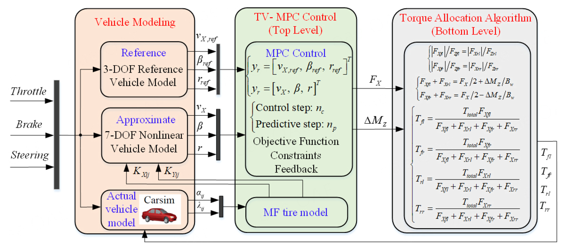
Figure 1. Structure of hierarchical control algorithm proposed herein.

The remainder of this paper is organized as follows. In Section 2, three models related to the vehicle are built. In Section 3, a time-varying MPC controller is designed. In Section 4 the equal-adhesion-rate-rule-based torque allocation algorithm is elaborated. In Section 5, the proposed method is demonstrated by conducting a Carsim–Simulink co-simulation. Finally, our concluding remarks are presented in Section 6.

2. VEHICLE MODEL

By considering the nonlinear and time-varying dynamic characteristics of 4WID EVs and the related control problems, an extended 3-DOF reference vehicle model and a nonlinear 7-DOF vehicle model are established in this section. In addition, a magic formula (MF) tire model is developed.

2.1. 3-DOF reference vehicle model

In this study, a single-track vehicle model is used as the 3-DOF reference vehicle model. According to[19], the actual and desired longitudinal accelerations of the vehicle satisfy the following first-order relationship:

$$ a = \frac{K}{1+\tau s} a_{des} $$

where $$ a $$ and $$ a_{des} $$ represent the actual and desired longitudinal accelerations of the vehicle, respectively; $$ K $$ = 1 is the system gain; and $$ \tau $$ is the time constant that ranges from 0.2 to 0.5. Therefore, the relationship between the actual and desired longitudinal velocities can be expressed as

$$ v_{X} = \frac{v_{X, des}}{1+\tau s} $$

Here, $$ v_{X, des} $$ can be calculated as follows:

$$ \dot{v}_{X, des} = \frac{F_{Xf}+F_{Xf}-F_{total}}{m} $$

where $$ m $$ denotes the vehicle mass; $$ F_{Xf} $$ and $$ F_{Xf} $$ denote the longitudinal front and rear tire forces, respectively; $$ F_{total} $$ is the total resistance force; and $$ v_{X, des} $$ and $$ v_{X, des} $$ denote the actual and desired longitudinal vehicle velocities, respectively. Combined with the traditional 2-DOF linear vehicle model, the transfer function of the 3-DOF reference vehicle model can be expressed as follows:

$$ \begin{eqnarray} \left\{\begin{array}{l} v_{X, ref} = v_{X, des} /(1+\tau s) \\ \beta_{ref} = G_{\beta, des} \delta_{f} /(1+Ts) \\ r_{ref} = G_{r_{r}, des} \delta_{f} /(1+Ts) \end{array}\right. \end{eqnarray} $$

where

$$ \large \begin{eqnarray*} \left\{\begin{array}{l} G_{\beta, d e s} = \frac{K_{f} K_{r} l_{r}\left(l_{f}+l_{r}\right)+m v_{X, des}^{2} K_{f} l_{f}}{K_{f} K_{r}\left(l_{f}+l_{r}\right)^{2}+\left(K_{f} l_{f}-K_{r} l_{r}\right) m v_{X, des}^{2}} \\ G_{r, des} = \frac{K_{f} K_{r}\left(l_{f}+l_{r}\right) v_{X, des}}{K_{f} K_{r}\left(l_{f}+l_{r}\right)^{2}+\left(K_{f} l_{f}-K_{r} l_{r}\right) m v_{X, des}^{2}} \\ T = \frac{m l_{f} v_{X, d e s}}{K_{r}\left(l_{f}+l_{r}\right)}-\frac{\left[m\left(K_{f} l_{f}^{2}+K_{r} l_{r}^{2}\right)+I_{Z}\left(K_{f}+K_{r}\right)\right] v_{X, des}}{K_{f} K_{r}\left(l_{f}+l_{r}\right)^{2}+\left(K_{f} l_{f}-K_{r} l_{f}\right) m v_{X, des}^{2}} \end{array}\right. \end{eqnarray*} $$

Here, $$ \delta_{f} $$ is the steering angle of the front wheel; $$ I_{Z} $$ is the yaw moment of the vehicle inertia; $$ l_{f} $$ and $$ l_{r} $$ are the distances from the mass center to the front and rear axles; $$ K_{f} $$ and $$ K_{r} $$ denote the front and rear wheel cornering stiffnesses; $$ \beta $$ and $$ r $$ are the sideslip angle and yaw rate of the vehicle, respectively.

2.2. 7-DOF nonlinear vehicle model

To obtain an accurate model for MPC control in the process of predicting the vehicle state, a 7-DOF nonlinear vehicle model, illustrated in Figure 2, is established, and it allows for free longitudinal motion, lateral motion, yaw motion, and rotation of the four wheels. The dynamic equilibrium equations of vehicle longitudinal, lateral, and yaw motions can be expressed as follows:

$$ \begin{eqnarray} \left\{\begin{array}{l} m\left(\dot{v}_{X}-r \beta v_{X}\right)=\left(F_{Xfl}+F_{Xfi}\right) \cos \delta_{f}+F_{Xrl}+F_{Xir}-\left(F_{Yfl}+F_{Yfi}\right) \sin \delta_{f} \\ m(\dot{\beta}+r) v_{X}=\left(F_{Xfl}+F_{Xfi}\right) \sin \delta_{f}+\left(F_{Yfl}+F_{Yfi}\right) \cos \delta_{f}+F_{Yrl}+F_{Yrr} \\ I_{Z} \dot{r}=\left(F_{Xfl}+F_{Xff}\right) l_{f} \sin \delta_{f}+\left[\left(F_{Xfi}-F_{Xf}\right) \cos \delta_{f}+\left(F_{Xir}-F_{Xrl}\right)\right] \frac{B_{w}}{2} \\ \quad+\left(F_{Yfl}+F_{Yff}\right) l_{f} \cos \delta_{f}+\left(F_{Yfl}-F_{Yfi}\right) \frac{B_{w}}{2} \sin \delta_{f}-\left(F_{Yrl}+F_{Y r r}\right) l_{r} \end{array}\right. \end{eqnarray} $$

Nonlinear hierarchical control for four-wheel-independent-drive electric vehicle

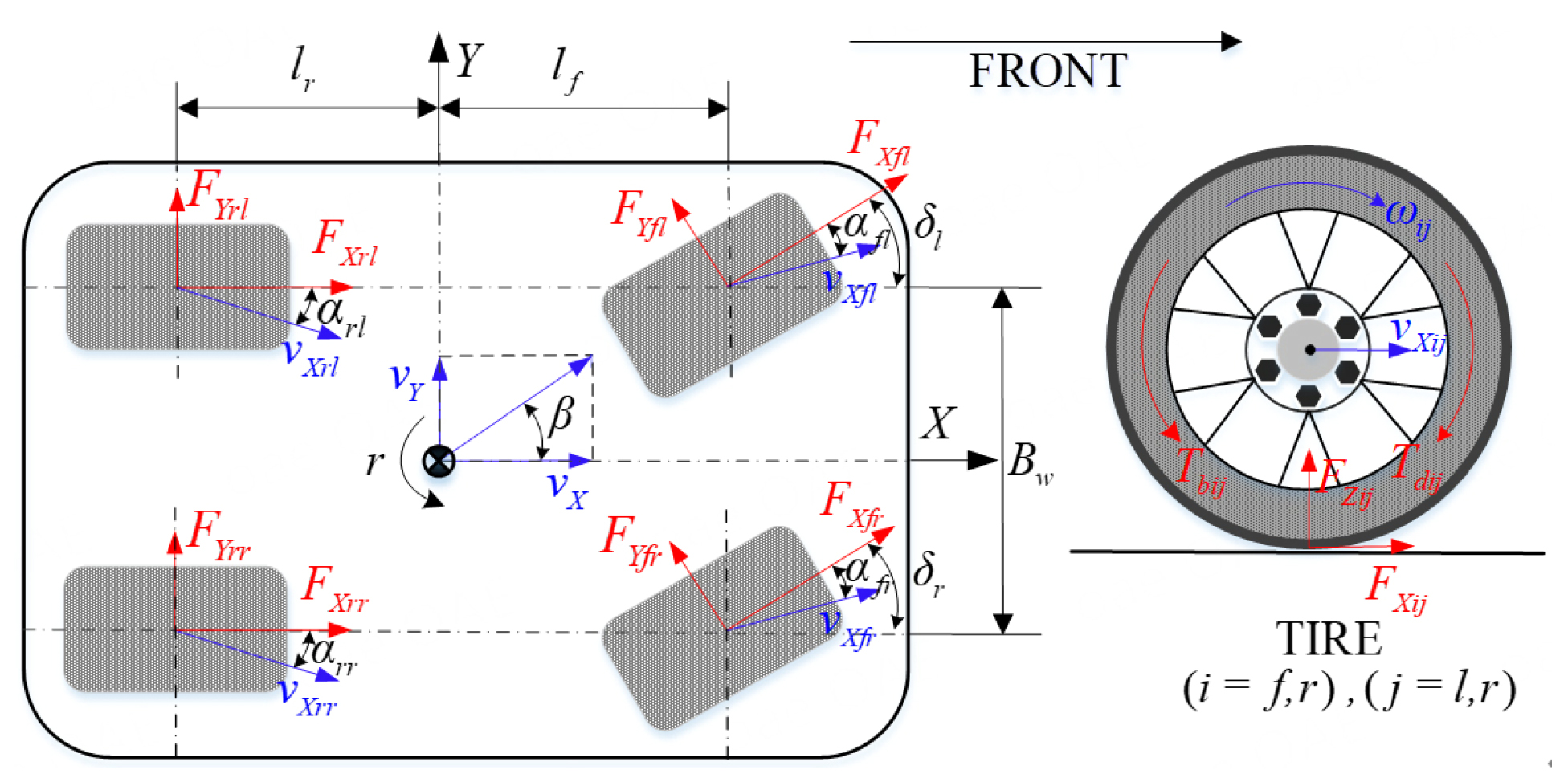
Figure 2. 7-DOF nonlinear vehicle dynamic model.

In this equation, $$ m $$ and $$ I_{Z} $$ denote the vehicle’s sprung mass and its moment of inertia around the Z axis, respectively; $$ B_{w} $$ is the vehicle’s wheelbase; $$ \delta_{f} $$ is the steering angle of the front axle, and it can be approximated as $$ \delta_{l} = \delta_{r} = \delta_{f} $$; $$ F_{Xij} $$ and $$ F_{Yij} $$ denote longitudinal and lateral tire forces (where $$ i = f $$ or $$ r $$, $$ j = l $$ or $$ r $$; $$ fl $$ means front left, $$ fr $$ means front right, $$ rl $$ means rear left, and $$ rr $$ means rear right), respectively. The meanings of the other parameters are given in Section 2.1.

The rotational dynamic equilibrium equation of each wheel is expressed as follows:

$$ I_{w} \dot{\omega}_{ij} = T_{ij}-F_{Xij} R_{w} \quad(i = f, r \quad j = l, r) $$

where $$ I_{w} $$ is the moment of wheel inertia around each axis of rotation, $$ R_{w} $$ is the effective radius of each wheel, $$ \omega_{ij} $$ denotes the rotation rate of each wheel, and $$ T_{ij} $$ is the driving torque $$ T_{dij} $$ or braking torque $$ T_{bij} $$ of each in-wheel motor.

MF tire model

The general form of the MF tire model[20] is as follows:

$$ Y(x) = D \sin \{C \arctan [B x-E(B x-\arctan (B x))]\} $$

where $$ x $$ is either the longitudinal slip ratio $$ \lambda_{ij} $$ or lateral slip angle $$ \alpha_{ij} $$. $$ B $$, $$ C $$, $$ D $$, and $$ E $$ denote the stiffness factor, shape factor, peak value, and curvature factor, respectively. The tire longitudinal slip ratio of each wheel is expressed as follows:

$$ \begin{eqnarray} \lambda_{ij} = \left\{\begin{array}{ll} \frac{\omega_{ij} R-v_{Xij}}{\omega_{ij} R_{w}} & \text { Driving Conditon } \\ \frac{v_{X_{ij}}-\omega_{ij} R}{v_{Xij}} & \text { Braking Conditon } \end{array}(i = f, r \quad j = l, r)\right. \end{eqnarray} $$

where $$ v_{Xxy} $$ denotes the longitudinal translational velocity of each wheel, which can be calculated as follows:

$$ \begin{eqnarray} \left\{\begin{array}{l} v_{Xfi}=\left(v_{X}-rB_{w}/ 2\right) \cos \delta_{f}+\left(v_{X} \beta+rl_{f}\right) \sin \delta_{f} \\ v_{Xfr}=\left(v_{X}+rB_{w}/2\right) \cos \delta_{f}+\left(v_{X} \beta+rl_{f}\right) \sin \delta_{f} \\ v_{Xrl}=v_{X}-r B_{w}/2\\ v_{Xrr}=v_{X}+r B_{w}/2 \end{array}\right. \end{eqnarray} $$

The tire lateral sideslip angle of each wheel can be expressed as follows:

$$ \begin{eqnarray} \left\{\begin{array}{ll} \alpha_{fl}=\frac{\beta v_{X}+r l_{f}}{v_{X}-r B_{w} / 2}-\delta_{f} \quad \quad \alpha_{r l}=\frac{\beta v_{X}-r l_{r}}{v_{X}-r B_{w} / 2} \\ \alpha_{fr}=\frac{\beta v_{X}+r l_{f}}{v_{X}+r B_{w} / 2}-\delta_{f} \quad \quad \alpha_{r r}=\frac{\beta v_{X}-r l_{r}}{v_{X}+r B_{w} / 2} \end{array}\right. \end{eqnarray} $$

The parameters $$ B $$, $$ C $$, $$ D $$, and $$ E $$ in the longitudinal MF tire model are given as follows:

$$ C=a_{0}, \quad D=\mu\left(a_{1} F_{Z}^{2}+a_{2} F_{Z}\right), \quad B=\left(a_{3} F_{Z}^{2}+a_{4} F_{Z}\right) e^{\sigma_{5} F_{z}} /(C D), \quad E=a_{6} F_{Z}^{2}+a_{7} F_{Z}+a_{8} $$

The parameters $$ B $$, $$ C $$, $$ D $$, and $$ E $$ in the lateral MF tire model are given as follows:

$$ C=b_{0}, \quad D=\mu\left(b_{1} F_{Z}^{2}+b_{2} F_{Z}\right), \quad B=b_{3} \sin \left[2 \arctan \left(F_{Z} / b_{4}\right)\right] /(C D), \quad E=b_{5} F_{Z}+b_{6} $$

where $$ a_{0} $$$$ a_{8} $$ and $$ b_{0} $$$$ b_{6} $$ can be calibrated by conducting tire force tests, and their values are listed in Table 1.

Table 1

MF tire model parameters $$ a_{0} $$$$ a_{8} $$ and $$ b_{0} $$$$ b_{6} $$

Parameter$$ a_{0} $$$$ a_{1} $$$$ a_{2} $$$$ a_{3} $$$$ a_{4} $$$$ a_{5} $$$$ a_{6} $$$$ a_{7} $$$$ a_{8} $$
Value1.37-0.00398.780.00765.1-0.0001600.00010.3
Parameter$$ b_{0} $$$$ b_{1} $$$$ b_{2} $$$$ b_{3} $$$$ b_{4} $$$$ b_{5} $$$$ b_{6} $$
Value1.388-0.04999.72, 3118.970.662-1, 323

$$ F_{Z} $$ is the tire vertical force, and the vertical force of each tire can be expressed as follows:

$$ \begin{eqnarray} \left\{\begin{array}{llll} F_{Zfl}=m_{w}g+mgl_{r}/\left(l_{f}+l_{r}\right)-m\dot{v}_{X}h/\left(l_{f}+l_{r}\right)-m(r+\dot{\beta})v_{X} hl_{r}/\left[B_{w}\left(l_{f}+l_{r}\right)\right] \\ F_{Zfr}=m_{w}g+mgl_{r}/\left(l_{f}+l_{r}\right)-m\dot{v}_{X}h/\left(l_{f}+l_{r}\right)+m(r+\dot{\beta})v_{X} hl_{r}/\left[B_{w}\left(l_{f}+l_{r}\right)\right] \\ F_{Zrl}=m_{w}g+mgl_{f}/\left(l_{f}+l_{r}\right)+m\dot{v}_{X}h/\left(l_{f}+l_{r}\right)-m(r+\dot{\beta}) v_{X} hl_{f}/\left[B_{w}\left(l_{f}+l_{r}\right)\right] \\ F_{Zrr}=m_{w}g+mgl_{f}/\left(l_{f}+l_{r}\right)+m\dot{v}_{X}h/\left(l_{f}+l_{r}\right)+m(r+\dot{\beta}) v_{X} hl_{f}/\left[B_{w}\left(l_{f}+l_{r}\right)\right] \end{array}\right. \end{eqnarray} $$

where $$ m_{w} $$ denotes tire mass, and $$ g $$ denotes gravitational acceleration. $$ h $$ is the distance between the roll center and sprung mass center. The longitudinal and lateral tire forces are limited in the adhesion ellipse. Therefore, the tire force calculated using the MF model can be modified using the following expressions:

$$ \begin{eqnarray} \left\{\begin{array}{ll} F_{X}=\frac{\left|\sigma_{X}\right|}{\sigma} Y(\lambda) & F_{Y}=\frac{\left|\sigma_{Y}\right|}{\sigma} Y(\alpha) \\ K_{X}=\frac{\partial F_{X}}{\partial \lambda} & K_{Y}=\frac{\partial F_{Y}}{\partial \alpha} \\ \sigma_{X}=\frac{\lambda}{1+\lambda} \quad \sigma_{Y}=\frac{\tan \alpha}{1+\lambda} & \sigma=\sqrt{\sigma_{X}^{2}+\sigma_{Y}^{2}} \end{array}\right. \end{eqnarray} $$

3. TIME-VARYING MPC

Model accuracy is the basis and key advantage of the MPC control method. To reflect the accuracy of the vehicle model to the extent possible, we utilize the nonlinear 7-DOF vehicle model developed in Section 2 as the basis of our MPC control strategy.

The longitudinal speed, sideslip angle, and yaw rate of the vehicle are set as the state variables of the predictive state space equation, which is expressed as $$ x=\left[v_{X}, \beta, r\right]^{T} $$. The longitudinal total force and the yaw moment due to differences between the longitudinal forces of the four tires are set as the control variables: $$ u=\left[F_{X}, \Delta M_{Z}\right]^{T} $$. The output variables of this system are the same as the state variables, that is, $$ y=\left[v_{X}, \beta, r\right]^{T} $$. The two control variables can be expressed approximately in terms of the longitudinal force of each tire, as follows:

$$ \begin{eqnarray} \left\{\begin{array}{l} F_{X}=F_{Xfl}+F_{Xfr}+F_{Xrl}+F_{Xrr} \\ \Delta M_{Z}=\left(F_{Xfr}-F_{Xfl}+F_{Xrr}-F_{Xrl}\right) B_{w} / 2 \end{array}\right. \end{eqnarray} $$

According to Eq. (5), the state-space representation of this control system is as follows:

$$ \dot{x}=f(x, u) $$

To reduce computational cost, the system state-space equation is linearized as follows:

$$ \begin{eqnarray} \left\{\begin{array}{l} \dot{x}=A x+B u \\ y=C x \end{array}\right. \end{eqnarray} $$

where

$$ A=\frac{\partial f(x, u)}{\partial x}=\left[\begin{array}{lll}\frac{\partial f}{\partial v_{X}} & \frac{\partial f}{\partial \beta} & \frac{\partial f}{\partial r}\end{array}\right], \quad B=\frac{\partial f(x, u)}{\partial u}=\left[\begin{array}{ccc}1 / m & 0 & 0 \\ 0 & 0 & 1 / I_{z}\end{array}\right]^{T}, \quad C=\operatorname{diag}(1, 1, 1) $$

$$ \begin{eqnarray} \frac{\partial f}{\partial v_{X}}=\left[\begin{array}{lll} r \beta+\frac{1}{m}\left[\left(\frac{\partial F_{Xfl}}{\partial v_{X}}+\frac{\partial F_{Xfr}}{\partial v_{X}}\right) \cos \delta_{f}+\frac{\partial F_{X r l}}{\partial v_{X}}+\frac{\partial F_{Xrr}}{\partial v_{X}}-\left(\frac{\partial F_{Yfl}}{\partial v_{X}}+\frac{\partial F_{Yfr}}{\partial v_{X}}\right) \sin \delta_{f}\right]; \\ \frac{1}{m v_{X}}\left[\left(\frac{\partial F_{Xfl}}{\partial v_{X}}+\frac{\partial F_{Xfr}}{\partial v_{X}}\right) \sin \delta_{f}+\left(\frac{\partial F_{Yfl}}{\partial v_{X}}+\frac{\partial F_{Yfr}}{\partial v_{X}}\right) \cos \delta_{f}+\frac{\partial F_{Yrl}}{\partial v_{X}}+\frac{\partial F_{Yrr}}{\partial v_{X}}\right] \\ -\frac{1}{m v_{X}^{2}}\left[\left(F_{Xfl}+F_{Xfr}\right) \sin \delta_{f}+\left(F_{Yfl}+F_{Yfr}\right) \cos \delta_{f}+F_{Yrl}+F_{Yrr}\right] ; \\ \frac{1}{I_{Z}}\left[\left(\frac{\partial F_{Xfl}}{\partial v_{X}}+\frac{\partial F_{Xfr}}{\partial v_{X}}\right) l_{f} \sin \delta_{f}+\left[\left(\frac{\partial F_{Xfr}}{\partial v_{X}}-\frac{\partial F_{Xfl}}{\partial v_{X}}\right) \cos \delta_{f}+\left(\frac{\partial F_{Xrr}}{\partial v_{X}}-\frac{\partial F_{Xrl}}{\partial v_{X}}\right)\right] \frac{B_{w}}{2}\right] \\ +\frac{1}{I_{Z}}\left[\left(\frac{\partial F_{Yfl}}{\partial v_{X}}+\frac{\partial F_{Yfr}}{\partial v_{X}}\right) l_{f} \cos \delta_{f}+\left(\frac{\partial F_{Yfl}}{\partial v_{X}}-\frac{\partial F_{Yfr}}{\partial v_{X}}\right) \frac{B_{w}}{2} \sin \delta_{f}-\left(\frac{\partial F_{Yrl}}{\partial v_{X}}+\frac{\partial F_{Yrr}}{\partial v_{X}}\right) l_{r}\right] \end{array}\right] \end{eqnarray} $$

$$ \begin{eqnarray*} \frac{\partial f}{\partial \beta}=\left[\begin{array}{lll} {r v_{X}+\frac{1}{m}\left[\left(\frac{\partial F_{Xfl}}{\partial \beta}+\frac{\partial F_{Xfr}}{\partial \beta}\right) \cos \delta_{f}+\frac{\partial F_{Xrl}}{\partial \beta}+\frac{\partial F_{Xrr}}{\partial \beta}-\left(\frac{\partial F_{Yfl}}{\partial \beta}+\frac{\partial F_{Yfr}}{\partial \beta}\right) \sin \delta_{f}\right] ;} \\ \frac{1}{m v_{X}}\left[\left(\frac{\partial F_{Xfl}}{\partial \beta}+\frac{\partial F_{Xfr}}{\partial \beta}\right) \sin \delta_{f}+\left(\frac{\partial F_{Yfl}}{\partial \beta}+\frac{\partial F_{Yfr}}{\partial \beta}\right) \cos \delta_{f}+\frac{\partial F_{Yrl}}{\partial \beta}+\frac{\partial F_{Yrr}}{\partial \beta}\right]; \\ \frac{1}{I_{z}}\left[\left(\frac{\partial F_{Xfl}}{\partial \beta}+\frac{\partial F_{Xfr}}{\partial \beta}\right) l_{f} \sin \delta_{f}+\left[\left(\frac{\partial F_{Xfr}}{\partial \beta}-\frac{\partial F_{Xfl}}{\partial \beta}\right) \cos \delta_{f}+\left(\frac{\partial F_{Xrr}}{\partial \beta}-\frac{\partial F_{Xrl}}{\partial \beta}\right)\right] \frac{B_{w}}{2}\right] \\ +\frac{1}{I_{z}}\left[\left(\frac{\partial F_{Yfl}}{\partial \beta}+\frac{\partial F_{Yfr}}{\partial \beta}\right) l_{f} \cos \delta_{f}+\left(\frac{\partial F_{Yfl}}{\partial \beta}-\frac{\partial F_{Yfr}}{\partial \beta}\right) \frac{B_{w}}{2} \sin \delta_{f}-\left(\frac{\partial F_{Yrl}}{\partial \beta}+\frac{\partial F_{Yrr}}{\partial \beta}\right) l_{r}\right] \\ \end{array}\right] \label{16b} \end{eqnarray*} $$

$$ \large \begin{eqnarray*} \frac{\partial f}{\partial r}=\left[\begin{array}{lll} \beta v_{X}+\frac{1}{m}\left[\left(\frac{\partial F_{Xfl}}{\partial r}+\frac{\partial F_{Xfr}}{\partial r}\right) \cos \delta_{f}+\frac{\partial F_{Xrl}}{\partial r}+\frac{\partial F_{Xrr}}{\partial r}-\left(\frac{\partial F_{Yfl}}{\partial r}+\frac{\partial F_{Yfr}}{\partial r}\right) \sin \delta_{f}\right] ; \\ -1+\frac{1}{m v_{X}}\left[\left(\frac{\partial F_{Xfl}}{\partial r}+\frac{\partial F_{Xfr}}{\partial r}\right) \sin \delta_{f}+\left(\frac{\partial F_{Yfl}}{\partial r}+\frac{\partial F_{Yfr}}{\partial r}\right) \cos \delta_{f}+\frac{\partial F_{Yrl}}{\partial r}+\frac{\partial F_{Yrr}}{\partial r}\right] ; \\ \frac{1}{I_{z}}\left[\left(\frac{\partial F_{Xfl}}{\partial r}+\frac{\partial F_{Xfr}}{\partial r}\right) l_{f} \sin \delta_{f}+\left[\left(\frac{\partial F_{Xfr}}{\partial r}-\frac{\partial F_{Xfl}}{\partial r}\right) \cos \delta_{f}+\left(\frac{\partial F_{Xrr}}{\partial r}-\frac{\partial F_{Xrl}}{\partial r}\right)\right] \frac{B_{w}}{2}\right] \\ +\frac{1}{I_{Z}}\left[\left(\frac{\partial F_{Yfl}}{\partial r}+\frac{\partial F_{Yfr}}{\partial r}\right) l_{f} \cos \delta_{f}+\left(\frac{\partial F_{Yfl}}{\partial r}-\frac{\partial F_{Yfr}}{\partial r}\right) \frac{B_{w}}{2} \sin \delta_{f}-\left(\frac{\partial F_{Yrl}}{\partial r}+\frac{\partial F_{Yrr}}{\partial r}\right) l_{r}\right] \end{array}\right] \label{16c} \end{eqnarray*} $$

The partial derivative in Eq. (15) can be calculated as follows:

$$ \large \left[\frac{\partial F_{Xij}}{\partial v_{X}} \frac{\partial F_{Xij}}{\partial \beta} \frac{\partial F_{Xij}}{\partial r}\right]=K_{Xij}\left[\begin{array}{lll} \frac{\dot{\lambda}_{Xij}}{\dot{v}_{X}} & \frac{\dot{\lambda}_{Xij}}{\dot{\beta}} & \frac{\dot{\lambda}_{Xij}}{\dot{r}} \end{array}\right] $$

$$ \large \begin{eqnarray*} {\left[\begin{array}{lll} \frac{\partial F_{Yfl}}{\partial v_{X}} & \frac{\partial F_{Yfl}}{\partial \beta} & \frac{\partial F_{Yfl}}{\partial r} \\ \frac{\partial F_{Yfr}}{\partial v_{X}} & \frac{\partial F_{Yfr}}{\partial \beta} & \frac{\partial F_{Yfr}}{\partial r} \\ \frac{\partial F_{Yrl}}{\partial v_{X}} & \frac{\partial F_{Yrl}}{\partial \beta} & \frac{\partial F_{Yrl}}{\partial r} \\ \frac{\partial F_{Yrr}}{\partial v_{X}} & \frac{\partial F_{Yrr}}{\partial \beta} & \frac{\partial F_{Yrr}}{\partial r} \end{array}\right]=\left[\begin{array}{llll} K_{Yfl} \frac{-r\left(\beta B_{w} / 2+l_{f}\right)}{\left(v_{X}-r B_{w} / 2\right)^{2}} & K_{Yfl} \frac{v_{X}}{v_{X}-r B_{w} / 2} & K_{Yfl} \frac{v_{X} l_{f}+\beta v_{X} B_{w} / 2}{\left(v_{X}-r B_{w} / 2\right)^{2}} \\ K_{Yfr} \frac{r\left(\beta B_{w} / 2-l_{f}\right)}{\left(v_{X}+r B_{w} / 2\right)^{2}} & K_{Yfr} \frac{v_{X}}{v_{X}+r B_{w} / 2} & K_{Yfr} \frac{v_{X} l_{f}-\beta v_{X} B_{w} / 2}{\left(v_{X}+r B_{w} / 2\right)^{2}} \\ K_{Yfl} \frac{-r\left(\beta B_{w} / 2-l_{f}\right)}{\left(v_{X}-r B_{w} / 2\right)^{2}} & K_{Yfl} \frac{v_{X}}{v_{X}-r B_{w} / 2} & K_{Yfl} \frac{-v_{X} l_{r}+\beta v_{X} B_{w} / 2}{\left(v_{X}-r B_{w} / 2\right)^{2}} \\ K_{Yfl} \frac{r\left(\beta B_{w} / 2+l_{f}\right)}{\left(v_{X}+r B_{w} / 2\right)^{2}} & K_{Yfl} \frac{v_{X}}{v_{X}+r B_{w} / 2} & K_{Yfl} \frac{-v_{X} l_{f}-\beta v_{X} B_{w} / 2}{\left(v_{X}+r B_{w} / 2\right)^{2}} \end{array}\right]} \\ \label{17b} \end{eqnarray*} $$

The parameters $$ K_{Xij} $$ and $$ K_{Yij} $$ can be obtained from the MF tire model by using Eq. (12). The parameters in matrix $$ A $$, which is detailed in Eqs. (16) and (17), can be expressed using the results of the $$ k $$-th step. Then, Eq. (15) can be discretized as follows:

$$ \begin{eqnarray} \left\{\begin{array}{l} x(k+1)=G(k) x(k)+H(T) u(k) \\ y(k)=C x(k) \end{array}\right. \end{eqnarray} $$

where

$$ \begin{eqnarray*} \left\{\begin{array}{l} G(k)=e^{A(k) T} \approx T A(k)+I \\ H(T)=\int_{0}^{T} e^{A T} d t \cdot B \approx T B \end{array}\right. \end{eqnarray*} $$

The discrete linear equation for MPC control can be rewritten in the following form:

$$ \begin{eqnarray} \left\{\begin{array}{l} \Delta x(k+1)=G(k) \Delta x(k)+H \Delta u(k) \\ y(k)=y(k-1)+C \Delta x(k) \end{array}\right. \end{eqnarray} $$

where $$ \Delta u(k)=u(k)-u(k-1) $$, and $$ \Delta x(k)=x(k)-x(k-1) $$. The predictive time domain of this system is composed of $$ n_{p} $$ steps, control time domain of this system is composed of $$ n_{c} $$ steps, and the relationship $$ n_{c} \leq n_{p} $$ holds. In this work, $$ n_{p} $$ and $$ n_{c} $$ are set to 8 and 3, respectively. The $$ n_{c} $$-step control input vector and $$ n_{p} $$-step predictive output vector can be expressed as follows:

$$ \begin{eqnarray} \left\{\begin{array}{l} \Delta U(k)=\left[\begin{array}{llll} \Delta u(k) & \Delta u(k+1) & \cdots & \Delta u(k+n_{c}-1) \end{array}\right]^{T} \\ Y(k)=\left[\begin{array}{llllll} y(k+1) & y(k+2) & \cdots & y(k+n_{c}) & \cdots & y(k+n_{p}) \end{array}\right]^{T}\\ \end{array}\right. \end{eqnarray}$$

Therefore, the output vector of each future predictive $$ n_{p} $$ steps is given as follows:

$$ Y(k)=S_{x}(k) x(k)+I_{y} y(k)+S_{u}(k) \Delta U(k) $$

where $$ S_{x}(k)=\left[\begin{array}{c}C G \\ \sum\limits_{i=1}^{2} C G^{i} \\ \vdots \\ \sum\limits_{i=1}^{n_{p}} C G^{i}\end{array}\right]_{(k)} $$, $$ I_{y}=\left[\begin{array}{c} I_{n_{c} \times n_{c}} \\ I_{n_{c} \times n_{c}} \\ \vdots \\ I_{n_{c} \times n_{c}} \end{array}\right]_{n_{p} \times 1} $$,

$$ S_{u}(k)=\left[\begin{array}{ccccc} C H & 0 & 0 & \cdots & 0 \\ \sum\limits_{i=1}^{2} C G^{i-1} H & C H & 0 & \cdots & 0 \\ \vdots & \vdots & \vdots & \ddots & \vdots \\ \sum\limits_{i=1}^{n_{c}} C G^{i-1} H & \sum\limits_{i=1}^{n_{c}-1} C G^{i-1} H & \cdots & \cdots & C H \\ \vdots & \vdots & \vdots & \ddots & \vdots \\ \sum\limits_{i=1}^{n_{p}} C G^{i-1} H & \sum\limits_{i=1}^{n_{p}-1} C G^{i-1} H & \cdots & \cdots & \sum\limits_{i=1}^{n_{p}-n_{c}+1} C G^{i-1} H \end{array}\right]_{(k)} $$

To track the reference vehicle model as well as possible, a 3-DOF vehicle model is designed as the reference model. According to Eq. (4), the reference discrete output vector can be obtained as follows:

$$ y_{r}(k)=G_{r}(T)y_{r}(k-1)+H_{r}(T)u_{r}(k-1) $$

where

$$ u_{r}(k)=\left[\begin{array}{lll} v_{X, d e s}(k) & \beta_{d e s}(k) & r_{d e s}(k) \end{array}\right]^{T}, \quad y_{r}(k)=\left[\begin{array}{lll} v_{X, r e f}(k) & \beta_{r e f}(k) & r_{r e f}(k) \end{array}\right]^{T} $$
,

$$ A_{r}=diag(1 / \tau, 1 / T, 1 / T), G_{r}(T)=I-T A_{r}, \text { and } H_{r}(T)=T A_{r} $$
. The $$ n_{p} $$-step predictive output vector of the reference system can be expressed as follows:

$$ Y_{r}(k)=\left[\begin{array}{llllll} y_{r}(k+1) & y_{r}(k+2) & \cdots & y_{r}(k+n_{c}) & \cdots & y_{r}(k+n_{p}) \end{array}\right]^{T} $$

Accordingly, the output vector of each future predictive $$ n_{p} $$ steps of the reference system is given as follows:

$$ Y_{r}(k)=W_{yr}y_{r}(k)+W_{ur}u_{r}(k) $$

where $$ W_{yr}=\left[\begin{array}{llll} G_{r} & G_{r}^{2} & \cdots & G_{r}^{n_{p}} \end{array}\right]^{T} $$, and $$ W_{ur}=\left[\begin{array}{llll} H_{r} & \sum\limits_{i-1}^{2} G_{r}^{i-1}H & \cdots & \sum\limits_{i-1}^{n_{p}} G_{r}^{i-1}H \end{array}\right]^{T} $$. In addition, the following relationship $$ u_{r}(k+1/k)=u_{r}(k)(i=1, 2 \cdots n_{p}) $$ holds.

The objective function of this MPC strategy has the following quadratic form:

$$ J(k)=\sum\limits_{i=1}^{n_{p}}\left\|y(k+i)-y_{r}(k+i)\right\|_{Q_{i}}^{2}+\sum\limits_{i=1}^{n_{e}}\|\Delta u(k+i-1)\|_{R_{i}}^{2}+\Theta $$

where $$ Q_{i} $$ and $$ R_{i} $$ are the weighting matrices of the first and second items, respectively. $$ \Theta $$ represents a positive relaxation factor. The objective of this function is to follow the ideal model smoothly and accurately. The first term of this function describes the ability of the actual vehicle model to track the reference model. The second term indicates the change in the input vector, which can restrict changes to the input variables. Meanwhile, the input, input increment, and output variables are constrained in a domain that can be expressed as follows:

$$ \begin{eqnarray} \left\{\begin{array}{l} u_{\min }(k+i) \leq u(k+i) \leq u_{\max }(k+i) \quad\left(i=0, 1, \cdots, n_{c}-1\right) \\ \Delta u_{\min }(k+i) \leq \Delta u(k+i) \leq \Delta u_{\max }(k+i) \quad\left(i=0, 1, \cdots, n_{c}-1\right) \\ y_{\min }(k+i) \leq y(k+i) \leq y_{\max }(k+i) \quad\left(i=0, 1, \cdots, n_{p}-1\right) \end{array}\right. \end{eqnarray} $$

Because of constraints, it is generally impossible to obtain the analytical solution to this problem. For this reason, it is necessary to transform it into a quadratic programming (QP) problem to obtain a numerical solution. Therefore, we convert the above constraint equations into the form $$ C_{Z}\ge b $$, as follows.

$$ \begin{eqnarray} \left\{\begin{array}{l} {\left[\begin{array}{c} -L_{\Delta U} \\ L_{\Delta U} \end{array}\right] \Delta U(k) \geq\left[\begin{array}{c} -\Delta U_{\max }(k) \\ \Delta U_{\min }(k) \end{array}\right]} \\ {\left[\begin{array}{c} -L_{U} \\ L_{U} \end{array}\right] \Delta U(k) \geq\left[\begin{array}{c} U^{\prime}(k-1)-U_{\text {max }}(k) \\ U_{\min }(k)-U^{\prime}(k-1) \end{array}\right]}\\ {\left[\begin{array}{c} -S_{u} \\ S_{u} \end{array}\right] \Delta U(k) \geq\left[\begin{array}{c} Y^{\prime}(k-1)-Y_{\max }(k) \\ Y_{\text {min }}(k)-Y^{\prime}(k-1) \end{array}\right]} \end{array}\right. \end{eqnarray}$$

where $$ L_{\Delta U} $$, $$ \Delta U_{\max }(k) $$, $$ \Delta U_{\min }(k) $$, $$ L_{U} $$, $$ U^{\prime}(k-1) $$, $$ U_{\max }(k) $$, $$ U_{\min }(k) $$, $$ Y^{\prime}(k-1) $$, $$ Y_{\max }(k) $$, and $$ Y_{\min }(k) $$ can be calculated according as described in[21]. Then, this question can be described as a standard QP problem. In this manner, the solution of this problem without the constraint equation can be set as the initial solution, which can be expressed as follows:

$$ \Delta U(k, 0)=\left(S_{u}^{T}(k-1) Q^{T} Q S_{u}(k-1)+R^{T} R\right) S_{u}^{T}(k-1) Q^{T} Q E(k) $$

where $$ E(k)=Y_{r}(k)-S_{x}(k-1) \Delta x(k)-I_{y} y(k) $$ he optimal solution of the input vector $$ \Delta U^{*}(k) $$ can be calculated using the algorithm of the QP problem with constraints. Then, the closed-loop control input can be obtained as follows:

$$ \Delta u(k)=\left[\begin{array}{llll} I_{2 \times 2} & 0 & \cdots & 0 \end{array}\right]_{1 \times n_{e}} \Delta U^{*}(k) $$

4. TORQUE ALLOCATION ALGORITHM

The proposed torque allocation algorithm based on the equal adhesion rate rule is described in this section. We adopt the equal adhesion rate rule by considering only the adhesion rate of longitudinal force because the deviations due to the lateral and longitudinal forces are excessive, meaning that no solution can be obtained. Therefore, the longitudinal forces on the left and right sides of the vehicle are expressed as follows.

$$ \begin{eqnarray} \left\{\begin{array}{l} \left|F_{Xfl}\right|/F_{Zfl}=\left|F_{Xrl}\right|/F_{Zrl} \\ \left|F_{Xfr}\right|/F_{Zfr}=\left|F_{Xrr}\right|/F_{Zrr} \end{array}\right. \end{eqnarray} $$

The total longitudinal forces on the left and right sides of the vehicle can be calculated as follows:

$$ \begin{eqnarray} \left\{\begin{array}{l} F_{Xfl}+F_{Xrl}=F_{X}/2+\Delta M_{Z}/B_{w} \\ F_{Xfr}+F_{Xrr}=F_{X}/2-\Delta M_{Z}/B_{w} \end{array}\right. \end{eqnarray} $$

Therefore, each longitudinal tire force can be solved quickly by using Eqs. (30) and (31). By using the solved longitudinal tire force and algorithm of equal-adhesion-rate-rule, the torque acting on each wheel can be determined as follows.

$$ \left\{\begin{array}{l} T_{fl}=\left(T_{total} F_{Xfl}\right) /\left(F_{Xfl}+F_{Xrl}+F_{Xfr}+F_{Xrr}\right) \\ T_{fr}=\left(T_{total} F_{Xfr}\right) /\left(F_{Xfl}+F_{Xrl}+F_{Xfr}+F_{Xrr}\right) \\ T_{rl}=\left(T_{total} F_{Xrl}\right) /\left(F_{Xfl}+F_{Xrl}+F_{Xfr}+F_{Xrr}\right) \\ T_{rr}=\left(T_{total} F_{Xrr}\right) /\left(F_{Xfl}+F_{Xrl}+F_{Xfr}+F_{Xrr}\right) \end{array}\right. $$

5. CO-SIMULATION AND RESULTS

To verify the proposed control algorithm, we compared it to the proportional-integral-derivative (PID) control strategy. The co-simulation method was used for this purpose. Two main typical driving conditions, namely $$ ① $$ double lane change (DLC) maneuver under high-adhesion-coefficient condition ($$ \mu $$ = 0.9) and $$ ② $$ DLC maneuver under low-adhesion-coefficient condition ($$ \mu $$ = 0.3), were considered. The parameters of the vehicle and in-wheel motors are summarized in Table 2.

Table 2

Parameters of vehicle and in-wheel motors

ParameterDescriptionValue/UnitParameterDescriptionValue/Unit
$$ m $$Vehicle mass812 kg$$ B_{w} $$Wheelbase1.65 m
$$ m_{w} $$Vehicle mass20 kg$$ P_{e} $$Rated power7.5 KW
$$ l_{f} $$Distance from mass center to front axle1.1 m$$ P_{m} $$Peak power12 KW
$$ l_{r} $$Distance from mass center to rear axle1.25 m$$ n_{e} $$Rated speed750 rpm
$$ I_{Z} $$Moment of vehicle inertia around Z axis808 kg $$ \cdot \text{m}^{2} $$$$ n_{m} $$Peak speed1, 000 rpm
$$ I_{w} $$Moment of tire inertia around rotation axis0.5 kg $$ \cdot \text{m}^{2} $$$$ T_{e} $$Rated torque150 Nm
$$ h $$Distance between roll center and center of sprung mass0.27 m$$ T_{m} $$Peak torque250 Nm
$$ R_{w} $$Distance between roll center and center of sprung mass0.29 m

The consistency of human driving cannot be guaranteed, and it would be unsuitable for real drivers to drive a vehicle at dangerously high speeds or on low-adhesion roads. For this reason, we conducted a simulation to validate the effectiveness of the proposed control scheme.

5.1. DLC maneuver on high-adhesion road

The adhesion coefficient on the high-adhesion road was set to 0.9, and the reference vehicle velocity was set to 100 km/h. Figure 3. depicts a comparison of the typical state parameters by using different control methods, which are without active control, hierarchical time-varying MPC control, and PID control. According to Figure 3A, the velocity fluctuation due to the proposed hierarchical time-varying MPC control was smaller than that due to PID control. As shown in Figure 3B, compared to the without active control and PID control methods, the hierarchical time-varying MPC control method decreased the maximum lateral displacement by approximately 0.25 m and 0.11 m, respectively. The yaw rate and sideslip angle of the vehicle under MPC control were able to follow the ideal curve furthest, which effectively enhanced vehicle handling stability and safety, as depicted in Figure 3C and D.

Nonlinear hierarchical control for four-wheel-independent-drive electric vehicle

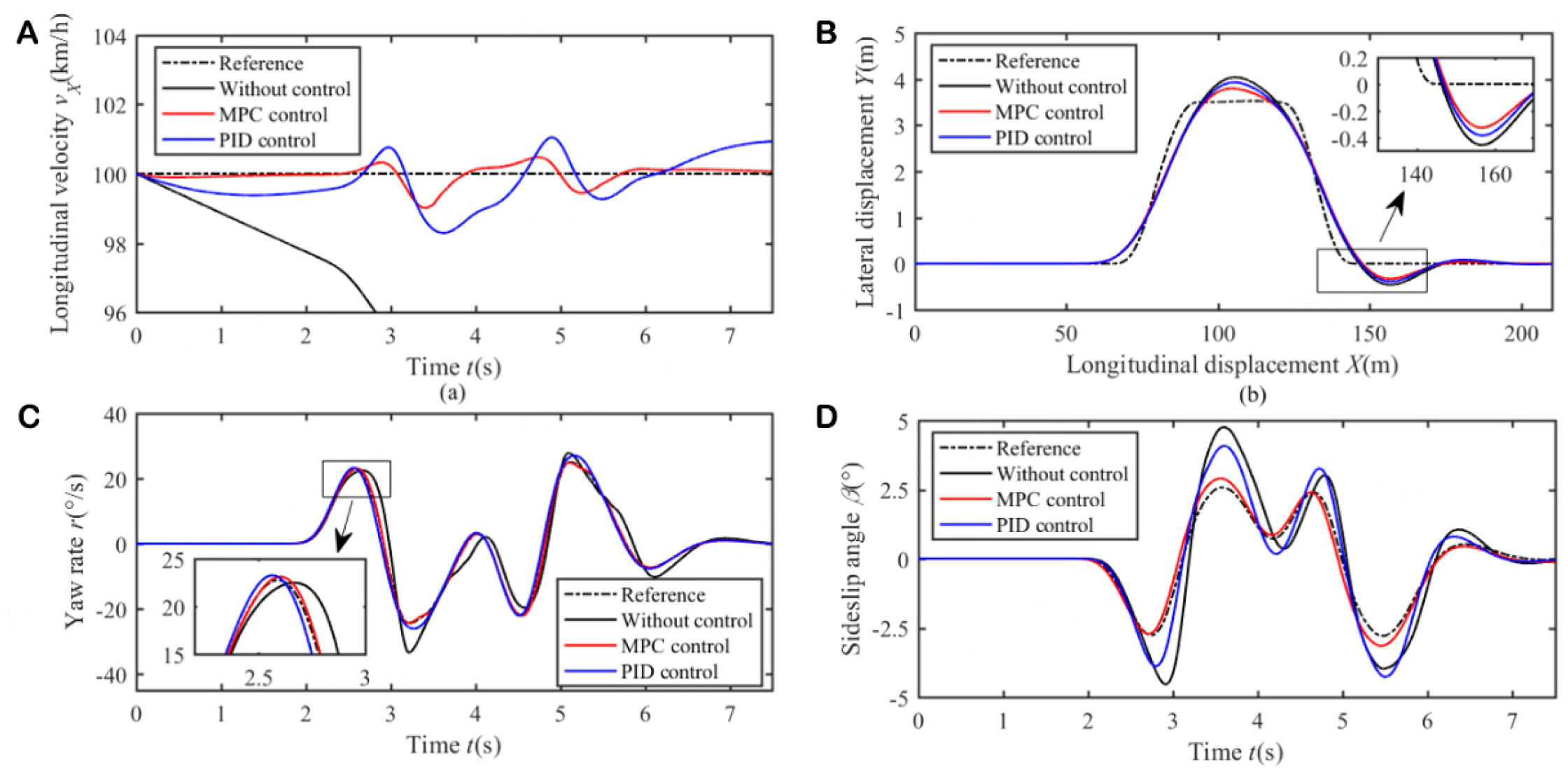
Figure 3. State comparison of different control modes during DLC maneuver. ($$ \mu $$ = 0.9, $$ v_{x} $$ = 100 km/h).

The adhesion rate can be expressed as follows:

$$ \varsigma_{ij}=\left|F_{Xij}\right| / F_{Zij} $$

where $$ i = f $$ or $$ r $$, $$ j = l $$ or $$ r $$, and $$ fl $$ denotes front left, $$ fr $$ denotes front right, $$ rl $$ denotes rear left, and $$ rr $$ denotes rear right.

The torque and adhesion rate of each tire are depicted in Figure 4. According to Figure 4A, the torque acting on each tire changed gently. Moreover, the torques acting on the left front and rear tires were similar but not equal. Likewise, the torques acting on the right front and rear tires were similar but not equal. However, the adhesion rates of the left two tires were almost equal, and the adhesion rates of the two right tires were almost equal, as depicted in Figure 4B. This indicates that the proposed algorithm can enhance vehicle safety and ensure that the adhesion rates of the two tires on the same side are as similar as possible.

Nonlinear hierarchical control for four-wheel-independent-drive electric vehicle

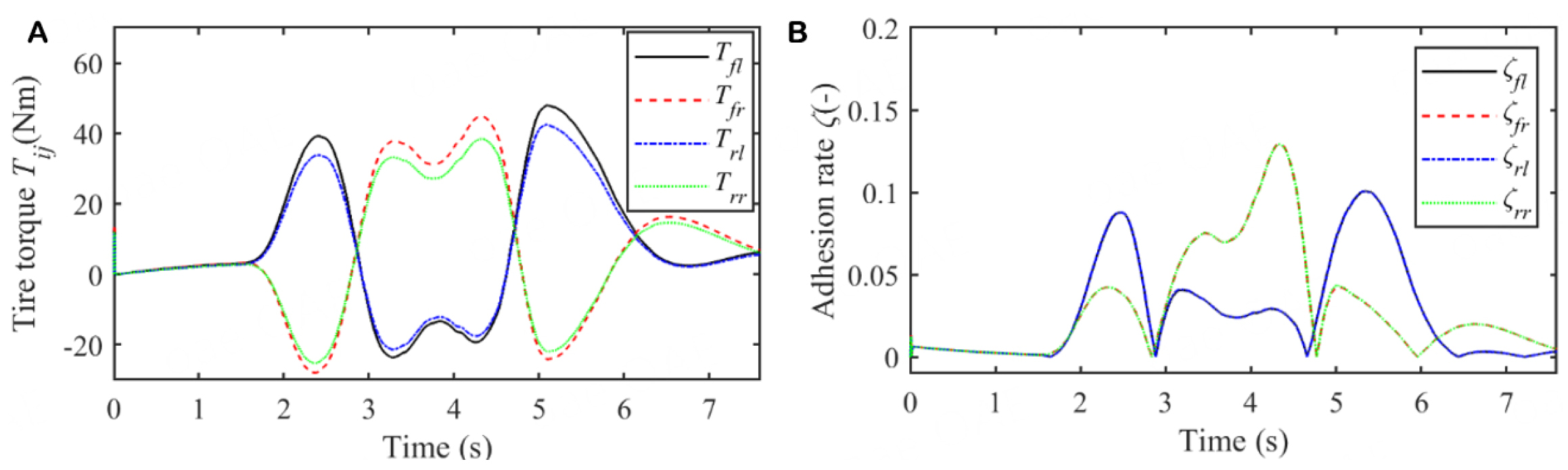
Figure 4. Torque and adhesion rate of each tire. ($$ \mu $$ = 0.9, $$ v_{x} $$ = 100 km/h).

5.2. DLC maneuver on low-adhesion road

Generally, a low-adhesion road can reflect the control effect more remarkably. The adhesion coefficient on a low-adhesion roads and the reference vehicle velocity were set to 0.3 and 70 km/h in this study. As illustrated in Figure 5A, the velocity fluctuation due to the hierarchical time-varying MPC control was smaller than that due to PID control, and with both methods, velocity fluctuations occurred close to the reference line. However, without control, the velocity dropped considerably. As shown inFigure 5B, the vehicle without control lost stability and deviated from the designated trajectory. The hierarchical time-varying MPC control reduced the maximum lateral displacement by approximately 0.2 m compared to that achieved with PID control. As depicted in Figure 5C and D, under hierarchical time-varying MPC control, the yaw rate and sideslip angle tracked the reference curves very well. The performance of PID control was slightly inferior in comparison, while the case without control performed the worst and the vehicle diverged from the set trajectory. With both PID control and hierarchical time-varying MPC control, the yaw rate control effect was stronger than the sideslip angle control effect because the sideslip angle is more difficult to control than the yaw rate. However, with hierarchical time-varying MPC control, the sideslip angle was less than $$ 2.5^\circ $$, which is within the safety limit.

Nonlinear hierarchical control for four-wheel-independent-drive electric vehicle

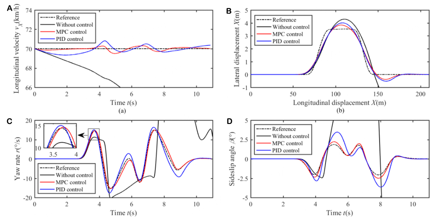
Figure 5. State comparison of different control modes during DLC maneuver ($$ \mu $$ = 0.3, $$ v_{x} $$ = 70 km/h).

The torque and adhesion rate of each tire are shown in Figure 6. According to Figure 6A, the torques acting on the left front and rear tires are similar but not equal, and the torques acting on the right front and rear tires are similar but not equal. However, the adhesion rates of the two left tires are almost equal, and the adhesion rates of the two right tires are almost equal, as shown in Figure 6B. This finding indicates that the proposed algorithm can secure vehicle safety and ensure that the adhesion rates of the two tires on the same side of the vehicle are as close to each other as possible. Unlike on the high-adhesion road, the torques and adhesion rates of each of the tires are lower, which is consistent with the actual situation.

Nonlinear hierarchical control for four-wheel-independent-drive electric vehicle

Figure 6. Torque and adhesion rate of each tire ($$ \mu $$ = 0.3, $$ v_{x} $$ = 70 km/h).

6. CONCLUSIONS

In this study, 3DOF reference vehicle model and a 7DOF nonlinear vehicle model were developed. A novel hierarchical time-varying MPC control strategy was proposed for 4WID EVs by considering vehicle stability and adhesion efficiency. A time-varying MPC controller was designed to reduce system error in the linearization process.

In the co-simulation, two typical conditions were adopted to demonstrate the performance of the proposed method. The DLC maneuver was performed on high- and low-adhesion roads to verify the effectiveness of the proposed control strategy. The results indicated that the proposed hierarchical time-varying MPC control strategy was able to enhance vehicle handling stability effectively. Furthermore, the lower torque allocation algorithm was able to improve the adhesion efficiency of each tire.

Declarations

Authors’ contributions

Conceptualization, methodology, writing-original Draft: Chen X

Supervision, project administration: Qu Y

Formal analysis: Cui T

Software, methodology: Zhao J

Availability of data and materials

Not applicable

Financial support and sponsorship

This work was supported by the National Natural Science Foundation of China (No. 52002211) and Key R&D Plan of Jiangsu Province (No. BE2022053-3).

Conflicts of interest

All authors declared that there are no conflicts of interest.

Ethical approval and consent to participate

Not applicable.

Consent for publication

Not applicable.

Copyright

© The Author(s) 2023.

REFERENCES

1. Zhuang W, Li S, Zhang X, et al. A survey of powertrain configuration studies on hybrid electric vehicles. Appl Energy 2020;262:114553.

2. Yang C, Shi Y, Li L, Wang X. Efficient mode transition control for parallel hybrid electric vehicle with adaptive dual-loop control framework. IEEE Trans Veh Technol 2020;69:1519-32.

3. Jing H, Jia F, Liu Z. Multi-objective optimal control allocation for an over-actuated electric vehicle. IEEE Access 2018;6:4824-33.

4. Liu J, Zhuang W, Zhong H, Wang L, Chen H, Tan C. Integrated energy-oriented lateral stability control of a four-wheel-independent-drive electric vehicle. Sci China Technol Sci 2019;62:2170-83.

5. Ma Y, Chen J, Zhu X, Xu Y. Lateral stability integrated with energy efficiency control for electric vehicles. Mech Syst Signal Process 2019;127:1-15.

6. Kobayashi T, Katsuyama E, Sugiura H, Ono E, Yamamoto M. Efficient direct yaw moment control: tyre slip power loss minimisation for four-independent wheel drive vehicle. Veh Syst Dyn 2018;56:719-33.

7. Zhao J, Wong PK, Ma X, Xie Z. Chassis integrated control for active suspension, active front steering and direct yaw moment systems using hierarchical strategy. Veh Syst Dyn 2017;55:72-103.

8. Song J. Active front wheel steering model and controller for integrated dynamics control systems. Int J Automot Technol 2016;17:265-72.

9. Zhang H, Wang J. Robust gain-scheduling control of vehicle lateral dynamics through AFS/DYC. In Modeling, dynamics and control of electrified vehicles. Amsterdam, The Netherlands: Elsevier; 2018. pp. 339-68.

10. Lenzo B, Bucchi F, Sorniotti A, Frendo F. On the handling performance of a vehicle with different front-to-rear wheel torque distributions. Veh Syst Dyn 2019;57:1685-704.

11. Ni J, Wang W, Hu J, Xiang C. Relaxed static stability for four-wheel independently actuated ground vehicle. Mech Syst Signal Process 2019;127:35-49.

12. Wu D, Ding H, Du C. Dynamics characteristics analysis and control of FWID EV. Int J Automot Technol 2018;19:135-46.

13. Chen Y, Hedrick JK, Guo K. A novel direct yaw moment controller for in-wheel motor electric vehicles. Veh Syst Dyn 2013;51:925-42.

14. Guo L, Ge P, Sun D. Torque Distribution Algorithm for Stability Control of Electric Vehicle Driven by Four In-Wheel Motors Under Emergency Conditions. IEEE Access 2019;7:104737-48.

15. Alipour H, Bannae Sharifian MB, Sabahi M. A modified integral sliding mode control to lateral stabilisation of 4-wheel independent drive electric vehicles. Veh Syst Dyn 2014;52:1584-606.

16. Chae M, Hyun Y, Yi K, Nam K. Dynamic Handling Characteristics Control of an in-Wheel-Motor Driven Electric Vehicle Based on Multiple Sliding Mode Control Approach. IEEE Access 2019;7:132448-58.

17. Hu C, Wang R, Yan F, Huang Y, Wang H, Wei C. Differential Steering Based Yaw Stabilization Using ISMC for Independently Actuated Electric Vehicles. IEEE Trans Intell Transport Syst 2018;19:627-38.

18. Peng H, Wang W, Xiang C, Li L, Wang X. Torque Coordinated Control of Four In-Wheel Motor Independent-Drive Vehicles With Consideration of the Safety and Economy. IEEE Trans Veh Technol 2019;68:9604-18.

19. Zhu M, Chen H, Xiong G. A model predictive speed tracking control approach for autonomous ground vehicles. Mech Syst Signal Process 2017;87:138-52.

20. Pacejka HB, Bakker E. The magic formula tyre model. Veh Syst Dyn 1992;21:1-18.

21. Camacho EF, Alba CB. Model predictive control. Springer Science & Berlin, Germany: Business Media, 2013.

Cite This Article

Export citation file: BibTeX | RIS

OAE Style

Chen X, Qu Y, Cui T, Zhao J. Nonlinear hierarchical control for four-wheel-independent-drive electric vehicle. Complex Eng Syst 2023;3:8. http://dx.doi.org/10.20517/ces.2022.50

AMA Style

Chen X, Qu Y, Cui T, Zhao J. Nonlinear hierarchical control for four-wheel-independent-drive electric vehicle. Complex Engineering Systems. 2023; 3(2): 8. http://dx.doi.org/10.20517/ces.2022.50

Chicago/Turabian Style

Chen, Xiang, Yuan Qu, Taowen Cui, Jin Zhao. 2023. "Nonlinear hierarchical control for four-wheel-independent-drive electric vehicle" Complex Engineering Systems. 3, no.2: 8. http://dx.doi.org/10.20517/ces.2022.50

ACS Style

Chen, X.; Qu Y.; Cui T.; Zhao J. Nonlinear hierarchical control for four-wheel-independent-drive electric vehicle. Complex. Eng. Syst. 2023, 3, 8. http://dx.doi.org/10.20517/ces.2022.50

About This Article

Special Issue

© The Author(s) 2023. Open Access This article is licensed under a Creative Commons Attribution 4.0 International License (https://creativecommons.org/licenses/by/4.0/), which permits unrestricted use, sharing, adaptation, distribution and reproduction in any medium or format, for any purpose, even commercially, as long as you give appropriate credit to the original author(s) and the source, provide a link to the Creative Commons license, and indicate if changes were made.

Data & Comments

Data

Views
738
Downloads
247
Citations
0
Comments
0
9

Comments

Comments must be written in English. Spam, offensive content, impersonation, and private information will not be permitted. If any comment is reported and identified as inappropriate content by OAE staff, the comment will be removed without notice. If you have any queries or need any help, please contact us at support@oaepublish.com.

0
Download PDF
Cite This Article 22 clicks
Like This Article 9 likes
Share This Article
Scan the QR code for reading!
See Updates
Contents
Figures
Related
Complex Engineering Systems
ISSN 2770-6249 (Online)

Portico

All published articles are preserved here permanently:

https://www.portico.org/publishers/oae/

Portico

All published articles are preserved here permanently:

https://www.portico.org/publishers/oae/