1.1. Context

Compliant control ^[1] has been widely employed to establish a stable and controlled interaction between a robot and the surrounding environment. While different implementations and approaches can be found in the state-of-the-art to deal with different applications ^[2-4], impedance and admittance controllers ^[5] are the most investigated strategies to deal with (partially) unknown environments ^[6-8]. While impedance control is suitable to control the interaction between the robot and a stiff environment, admittance control performs better when the robot interacts with a soft environment ^[9]. Indeed, a control framework capable of combining both controllers would improve the interaction control performance. It would allow switching between the right behavior for the interaction control considering soft environments (or free motion phases, in which the environment stiffness can be considered null) and for the interaction control considering stiff environments. Even though the modulation of such control behaviors has been addressed by the variable impedance control (i.e., to tune the controller parameters to deal with different environments/task phases ^{[10, 11]}), hybrid control frameworks have also been developed to combine the capabilities of both impedance and admittance controllers. In the following, the state-of-the-art hybrid controllers are analyzed to highlight the related open issues.

1.2. Related works

The complementary performance of impedance and admittance controllers is qualitatively shown in Figure 1. A hybrid controller that combines the behaviors of both impedance and admittance control would result in improved interaction control performance and would allow implementing a generalized interaction controller capable of dealing with any interaction environment.

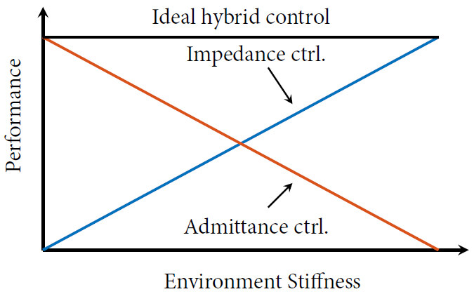
Figure 1. Qualitative complementarity of impedance and admittance controllers performance.

Ott et al.^[12] summarized the hybrid control framework in ^{[12, 13]}, which enhances the performance of interaction control in the whole spectrum of environment stiffness values. The proposed approach consists of applying the impedance and admittance controllers alternatively by exploiting a switching mechanism defined by a switching period parameter $$ \delta $$ (which is the time the impedance control and the admittance control are alternatively applied to the robot controller) and by a duty cycle parameter $$ n\in[0, 1] $$ (that determines the portion of $$ \delta $$ assigned to the impedance and the admittance controllers, $$ (1-n)\delta $$ and $$ n\delta $$, respectively). Simulated and experimental results were provided for a one-degree-of-freedom (DoF) robot. Successively, Cavenago et al.^[14] and Mei et al.^[15] applied the hybrid control framework on a simulated $$ 2 $$ DoF robot. Cavenago et al.^[14] introduced a neural network (NN) for the choice of $$ n $$, considering as an input to the NN the robot position and velocity and the external forces, while Mei et al.^[15] introduced a damping term $$ D_{env} $$ into the model of the environment. In addition, the optimal duty cycle parameter $$ n $$ is identified as a function of the environmental stiffness $$ K_{env} $$ and damping $$ D_{env} $$ parameters. This showed how the optimal $$ n $$ is not associated with the external stiffness in a unique way. Izadbakhsh et al.^[16] proposed an adaptive impedance controller using function approximation techniques where the system uncertainties are represented as basis functions and the aim is to converge to target impedance parameters with lower computational requirements. Other approaches have been proposed for the definition of a hybrid controller, such as the event-based hybrid controller by Yang et al.^[17] or the Maxwell model-based controller proposed by Fu et al.^[18]. However, the performance achieved by such approaches is not comparable to the ones achieved by the switching logic-based approaches. This paper aims to modify the approach of Ott et al.^[13] in order to further improve its performance. In particular, considering the approaches in ^[13-15], the inertia parameters of the models considered for the robot simulation were of the order of $$ 1 $$ kg. Moreover, the $$ 2 $$ DoF controlled robot in ^{[14, 15]} moved in the neighborhood of its equilibrium position, i.e., where the inertia matrix $$ {\bf{M}}_x({\bf{q}}) $$ of the robot can be considered as constant. However, the inertia parameter affects the definition of the switching parameter $$ \delta $$ and the duty cycle $$ n $$. Indeed, the adaptation of such parameters as a function of the robot inertia needs to be considered in order to optimize the performance of the hybrid controller (i.e., the combined behavior of impedance and admittance controllers). In addition, the improvement of the switching conditions (from impedance to admittance control) can be addressed in order to guarantee the continuity (i.e., the smoothness) of the interaction force. The main goal of the proposed paper is to address these issues.

1.3. Paper Contribution

Based on the discussion provided in the previous section, the main goals of the proposed paper are as follows:

(i) Satisfy the continuity of the interaction force in switching from impedance to admittance control when a feedforward velocity term is present.

(ii) Adapt the switching parameters to improve the performance of the hybrid control framework, thus better exploiting the properties of both impedance and admittance controllers.

While Aim (i) is addressed by the definition of proper initialization conditions at the switching time from impedance to admittance control taking into account a feedforward velocity term; Aim (ii) is addressed by adapting the switching parameters on the basis of the resulting robot inertia parameter (for the adaptation of the switching parameter $$ \delta $$) and the environment stiffness parameter (for the adaptation of the duty cycle $$ n $$).

The implemented methodologies were evaluated in simulation in Matlab, making use of a Franka EMIKA panda robot as a reference robotic platform, comparing the achieved results with respect to the standard method, which uses $$ \delta_i $$ fixed and an adaptation law for $$ n $$ as Ott et al.^[13], to demonstrate the improved performance (i.e., improved performance of the combined impedance/admittance controllers during interaction with a variable stiffness environment).

1.4. Paper outline

The paper is structured as it follows. Section 2 describes the hybrid controller of Ott et al.^[13], together with the low-level controller (i.e., impedance and admittance controllers). Section 3 introduces the modified hybrid control framework in order to deal with the discussed open issues of the state-of-the-art. Section 4 shows the achieved results of the proposed modified hybrid controller with respect to the one using $$ \delta_i $$ fixed and an adaptation law for $$ n $$ as in Ott et al.^[13]. Section 5 states the conclusions of the paper.

2.1. Robot dynamics modeling and control design

To design the impedance and admittance controllers, the robot dynamics can be modeled as follows ^[19]:

where $$ {\bf{q}} $$, $$ \dot{{\bf{q}}} $$, and $$ \ddot{{\bf{q}}} $$ are, respectively, the joint position, velocity, and acceleration vectors, $$ {\bf{M}}({\bf{q}}) $$ is the inertia matrix, $$ {\bf{C}}({\bf{q}}, \dot{{\bf{q}}}) $$ is the Coriolis and centrifugal matrix, $$ {\bf{G}}({\bf{q}}) $$ is the gravitational vector, and $$ \mathit{\boldsymbol{\tau}}_{F} $$ is the joint friction torques vector. $$ \mathit{\boldsymbol{\tau}}_{env} $$ represents the external interaction projected in the joint space (i.e., external interaction torques). $$ \mathit{\boldsymbol{\tau}}_{ctrl} $$ is the control torque vector, which is computed based on the impedance (i.e., $$ \mathit{\boldsymbol{\tau}}_{IMP} $$) or the admittance (i.e., $$ \mathit{\boldsymbol{\tau}}_{ADM} $$) control strategy, in addition to the following robot dynamics compensation term $$ \mathit{\boldsymbol{\tau}}_{dyn} $$:

where $$ {\bf{F}}_{CTRL} $$ is defined as the impedance (i.e., $$ {{\bf{F}}_{IMP}} $$) or the admittance (i.e., $$ {{\bf{F}}_{ADM}} $$) control force.

2.2. Impedance control

The Cartesian impedance control can be defined as it follows ^[19]:

$$ {\bf{M}}_x({\bf{q}}) $$ and $$ {\bf{C}}_x({\bf{q}}, \dot{{\bf{q}}}) $$ are defined as in Equation (5) and in Equation (6), respectively:

where $$ {\bf{J}}_{A} $$ defines the Jacobian matrix and $$ ^{\dagger} $$ its pseudo-inverse. The impedance control torque $$ \mathit{\boldsymbol{\tau}}_{IMP} $$ is then defined as follows:

2.3. Admittance control

The admittance control generates a position reference $$ {\bf{x}}_d $$ to be tracked by an inner position controller based on the following target dynamics ^[19], slightly modifying the controller in Equation (1):

where $$ {\bf{e}}_{d}={\bf{x}}_d-{\bf{x}}_0 $$ is the tracking error of the admittance controller. The computed position reference $$ {\bf{x}}_d $$ is then sent to the inner position controller to perform the tracking of the position error $$ {\bf{x}} - {\bf{x}}_d $$, providing the admittance control wrench $$ {\bf{F}}_{ADM} $$:

where $$ {\bf{K}}_p $$ and $$ {\bf{K}}_v $$ are the inner position control gain matrices and $$ \tilde{{\bf{e}}}_d={\bf{x}} - {\bf{x}}_d= {\bf{x}} - ({\bf{x}}_0 + {\bf{e}}_d) $$. The admittance control torque $$ \mathit{\boldsymbol{\tau}}_{ADM} $$ is then defined as follows:

2.4. Hybrid impedance/admittance control

The hybrid impedance/admittance control can be implemented on the basis of the approach proposed by Ott et al.^[12], so that it would be possible to exploit the combined performance of both control schema to deal with a wide range of interaction environment stiffnesses. The proposed hybrid controller continuously switches between impedance and admittance control. For this purpose, the switching period $$ \delta $$ and the duty cycle $$ n \in [0, 1] $$ parameters are introduced as control variables. The control force $$ {\bf{F}}_{CTRL} $$ is, therefore, computed according to the following strategy:

where $$ k $$ is an integer taking values $$ 0, 1, ... $$.

In Equation (11), $$ {\bf{F}}_{IMP} $$ and $$ {\bf{F}}_{ADM} $$ are computed, respectively, as described in Sections 2.2 and 2.3. As $$ n $$ approaches $$ 0 $$, $$ {\bf{F}}_{CTRL} $$ is equivalent to the impedance control action, while, as $$ n $$ approaches $$ 1 $$, $$ {\bf{F}}_{CTRL} $$ is equivalent to the admittance control action with periodic resetting. The hybrid impedance/admittance control framework is schematized in Figure 2.

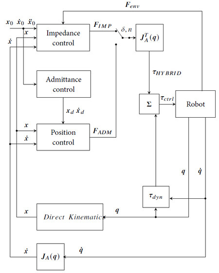
Figure 2. Hybrid impedance/admittance control schema.

While the hybrid impedance/admittance control proposed by Ott et al.^[13] provides a useful control framework to combine the impedance control and admittance control performance, the following main open issues are still present in the state-of-the-art: (i) the switching law to ensure continuity in the switching from impedance to admittance control does not include a feed-forward velocity term; and (ii) the performance of the hybrid impedance/admittance control framework (i.e., the resulting combined impedance/admittance behavior) can be improved by adapting the switching parameters that were considered constant by Ott et al.^[13]. In the following section, these open issues are tackled to improve the hybrid impedance/admittance control framework.

3.1. Proper initialization of the admittance controller

To guarantee the continuity of the interaction force while switching from impedance control to admittance control within the hybrid controller, the proper initialization of $$ {{\bf{e}}}_{d}(t_{sw}) $$ and $$ \dot{{\bf{e}}}_{d}(t_{sw}) $$ in Equation (9) has to be performed. In this section, three different methods are proposed to solve the mentioned issue: (i) the algebraic switching method; (ii) the differential switching method; and (iii) the iterative switching method.

3.1.3. Iterative switching method

Equation (12) shows that there are infinite combinations of $$ {{e}}_{d, i}(t_{sw}) $$ and $$ {\dot{e}}_{d, i}(t_{sw}) $$ so that $$ F_{IMP, i}=F_{ADM, i} $$ at $$ t_{sw} $$. However, only one of these pairs guarantees the continuity of the time derivative. An iterative methodology can be proposed to optimize $$ {{e}}_{d, i}(t_{sw}) $$ and $$ {\dot{e}}_{d, i}(t_{sw}) $$, as shown in algorithm 1. Given a user-defined tolerance on $$ \Delta \dot{F}=|\dot{F}_{ADM, i}-\dot{F}_{IMP, i}| $$, the proposed approach optimizes $$ {{e}}_{d, i}(t_{sw}) $$ and $$ {\dot{e}}_{d, i}(t_{sw}) $$. It is possible to use the results obtained from the algebraic method as first guesses for $$ {{e}}_{d, i}(t_{sw}) $$ and $$ {\dot{e}}_{d, i}(t_{sw}) $$. Figure 3 shows the convergence of the algorithm, being fast and feasible for online implementation. The convergence of the proposed approach depends on the tolerance of $$ |\dot{F}_{ADM, i}-\dot{F}_{IMP, i}| $$, as shown in Figure 4.

Algorithm 1

Iterative switching method algorithm.

$$ jj=1 $$
$$ toll=0.001 $$
$$ step=0.02 $$
$$ t_{sw}=t_{IMP_i \rightarrow ADM_i} $$
$$ \dot{F}_{IMP, i}=\frac{F_{IMP, i}(t_{sw})-F_{IMP, i}(t_{sw}-dt)}{dt} $$
$$ \dot{F}_{ADM, i}=K_{p, i}({\dot{e}}_{d, i}(t_{sw})+\dot{x}_{0, i}(t_{sw})-\dot{x}_i(t_{sw}))+K_{v, i}({\ddot{e}}_{d, i}(t_{sw})+\ddot{x}_{0, i}(t_{sw})-\ddot{x}_i(t_{sw}))+\dot{K}_{v, i}(t_{sw})({\dot{e}}_{d, i}(t_{sw})+\dot{x}_{i, 0}(t_{sw})-\dot{x}_i(t_{sw})) $$
$$ err=|\dot{F}_{ADM, i}-\dot{F}_{IMP, i}| $$
$$ state=up $$

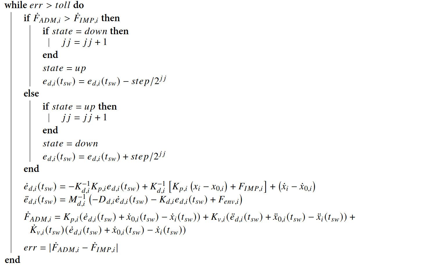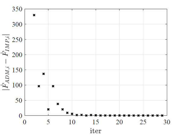
Figure 3. Convergence of the proposed iterative switching method considering the error $$ |\dot{F}_{ADM, i}-\dot{F}_{IMP, i}| $$.

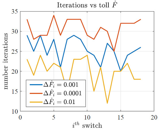
Figure 4. Switching iteration for the given tolerance value on $$ \Delta \dot{F}_i=|\dot{F}_{ADM, i}-\dot{F}_{IMP, i}| $$. As can be seen, the algorithm is stopped based on the defined tolerance.

3.2. Adaptive switching logic

The switching logic is defined by the following two parameters: the switching period $$ \delta $$ and the duty cycle $$ n $$. As shown in ^[13], such parameters affect the performance of the hybrid impedance/admittance controller. In particular, based on the equivalent inertia of the controlled robot along the direction $$ i $$, the switching parameters have to be adapted in order to maximize the performance of the hybrid controller. As shown in Figure 5 (considering the $$ z $$ DoF) for the Franka EMIKA panda robot (i.e., the robot used for the simulation results analysis in Section 4), the equivalent inertia $$ {\bf{M}}_x({\bf{q}}) $$ Equation (5) of the controlled robot (analysis performed exploiting the modeled robot dynamics in ^[20]) varies in a wide range based on the robot configuration. Indeed, to improve the performance of the hybrid controller, such an inertia variation has to be considered for the adaptation of the switching parameters. To support the above discussion, the modification of the achieved hybrid control performance can be seen in Figure Figure 6a, 6b, 6c for the the algebraic, differential, and iterative switching method, respectively, on the basis of the imposed value for the switching parameter $$ \delta $$, where the environmental stiffness behaves as shown in Figure Figure 6d. The robot interacts with the target environment along the vertical $$ z $$ direction, moving the setpoint down from its initial positioning of $$ 0.05 $$ m. As shown in the figure, the switching parameter value allows modulating the impedance/admittance combined behavior. For low values of $$ \delta $$, the controller behaves very similarly to the impedance controller even if $$ n=0.5 $$, for which an intermediate behavior is desirable. As $$ \delta $$ increases, the hybrid controller behaves as the admittance controller. In addition, when $$ \delta $$ increases too much, some undesirable oscillations are introduced. Therefore, the optimization of the switching parameter $$ \delta $$ would allow improving the hybrid controller performance. In addition, the adaptation of the duty cycle parameter $$ n $$ can be performed. As shown in ^{[13, 14]}, the duty cycle $$ n $$ can be adapted on the basis of the environment stiffness parameter. Indeed, this paper proposes a strategy to adapt such a parameter in order to improve the performance of the hybrid controller.

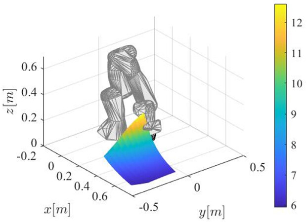
Figure 5. Cartesian equivalent inertia $$ {\bf{M}}_x({\bf{q}}) $$ along the $$ z $$ DoF as a function of the robot configuration for the considered Franka EMIKA panda robot

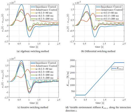
Figure 6. Hybrid control performance on the basis of the switching parameter $$ \delta $$ values for all the initialization methodologies for switching from impedance to admittance control.

In the following, the adaptation of both the switching period $$ \delta $$ and the duty cycle $$ n $$ are tackled to improve the hybrid control performance.

3.2.1. Variable switching period $$ \delta $$

To tune the switching period $$ \delta_i $$ on the basis of the inertia value along a specified Cartesian DoF $$ i $$, the following adaptation strategy has been defined:

(17) $$ \begin{equation} \delta_i=\delta_{0, i}\left(\frac{m_i}{m_{0, i}}\right)^{a_i}, \end{equation} $$

where $$ \delta_{0, i} $$ is the nominal value for the switching parameter, given a nominal inertia $$ m_{0, i} $$, while $$ m_i $$ is the current inertia value resulting from Equation (5) along a specified DoF $$ i $$. $$ a_i $$ is the parameter tuning the adaptation strategy in Equation (17).

To tune the $$ a_i $$ parameter, simulations can be exploited, as in Ott et al.^[13]. By introducing the performance index $$ p_{ref} $$ for the hybrid controller with a given value of the duty cycle $$ n $$,

(18) $$ \begin{equation} p_{ref, i}\vert_{n_i}=n_i p\vert_{IMP, i}+(1-n_i)p\vert_{ADM, i}, \end{equation} $$

where $$ p\vert_{IMP, i} $$ and $$ p\vert_{ADM, i} $$ are the performance for the pure impedance and admittance, respectively, as defined below in Equation (20), the following cost function can be defined for the optimization of $$ a_i $$,

(19) $$ \begin{equation} C_{env, n_i, i}=\int_{0}^{t_{f}} \left(p_{ref, i}\vert_{n_i, env}-p_i\vert_{n_i, env}\right)^2 \, dt, \end{equation} $$

for a given interaction environment $$ _{env} $$, where

(20) $$ \begin{equation} p_{ref, i}=(x_i-x_{ref, i})\vert_{m_i=m_{0, i}, \delta_i=\delta_{0, i}}, \\ p_i=(x_i-x_{ref, i})\vert_{m_i, \delta_i}. \end{equation} $$

By simulating the interaction with different environments (i.e., having different stiffness) and values of the duty cycle $$ n $$, it is possible to define the global cost function $$ C_i $$ and the partial ones $$ C_{env, i} $$ w.r.t the chosen environmental stiffness, as follows:

(21) $$ \begin{equation} C_i=\sum\limits_{env} \sum\limits_{n_i}C_{env, n_i, i}, \quad C_{env, i}= \sum\limits_{n_i} C_{env, n_i, i}. \end{equation} $$

To evaluate the cost function $$ C_i $$, a nominal inertia $$ m_{0, i}=1 $$ kg and a nominal switching parameter $$ \delta_{0, i}=20 $$ ms as considered by Ott et al.^[13], having the hybrid controller in interaction with soft, medium, and stiff environments with stiffness values of $$ 10 $$, $$ 300 $$, and $$ 3200 $$ N/m, respectively, were considered.

Figure 7 shows the cost functions $$ C_i $$ and $$ C_{env, i} $$ for a specified value of the inertia parameter $$ m_i $$, and varying the $$ \delta_i $$ parameter. Figure Figure 8a, 8b, 8c shows which value of $$ \delta_i $$ is the best when the system interacts with soft, medium, and stiff environments, respectively, for several values of inertia $$ m_i $$ (i.e., making it possible to highlight the optimized $$ \delta_i $$ parameter for every environment for the considered values of $$ m_i $$, as in Figure Figure 8d). Figure 9 collects the minimums of the cost functions highlighted in Figure 8a, 8b, 8c, 8d. It is then possible to optimize the value of $$ a_i $$ such that Equation (17) approximates the behavior of $$ \delta $$ in Figure 9. The optimized value of $$ a_i $$ is $$ 0.68 $$ (taking into consideration the target inertia range, in this case from +50% to $$ - $$20% w.r.t. $$ m_{0, i} $$). It follows that, if the inertia varies with respect to its nominal value, the value of $$ \delta_i $$ will increase with the law defined in Equation (17).

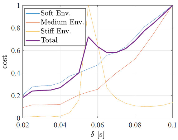
Figure 7. Contributions to the cost function for the soft, medium, and stiff environments, considering an inertia parameter $$ m_i=0.8 $$ kg and varying the $$ \delta_i $$ parameter.

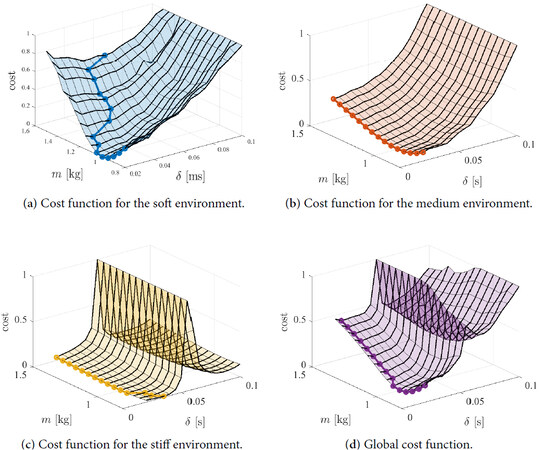
Figure 8. Normalized cost functions for soft, medium, and stiff environments and total normalized cost. The minimum for every value of the inertia $$ m_i $$ parameter is highlighted.

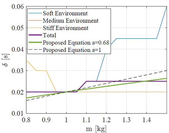
Figure 9. $$ \delta $$ corresponding to the minimum of the cost function for a given value of the inertia.

It has to be noted that the optimized value of $$ a_i $$ depends on the nominal parameters $$ m_{0, i} $$ and $$ \delta_i $$, together with the considered range of variation for $$ m_i $$. Therefore, changing, e.g., the range of variation for $$ m_i $$, a new optimization has to be performed.

3.2.2. Variable duty cycle $$ n $$

The adaptation of the duty cycle parameter $$ n $$ can be performed on the basis of the environmental stiffness parameters as it follows:

(22) $$ \begin{equation} n_i= \begin{cases} \hphantom{spazio}0&: K_{env, i}\in {\rm{soft \;environment}}, \\ \frac{K_{env, i}^{max}-K_{env, i}}{K_{env, i}^{max}-K_{env, i}^{min}}&: K_{env, i}\in {\rm{medium\; environment}}, \\ \hphantom{spazio}1&: K_{env, i}\in {\rm{stiff\; environment}}.\\ \end{cases} \end{equation} $$

This means that, when interacting with a soft environment (i.e., $$ n_i=0 $$), the controller is imposed to behave as the admittance controller; when interacting with a stiff environment (i.e., $$ n_i=1 $$), the controller is imposed to behave as the impedance controller; and when interacting with a medium environment, the duty cycle $$ n_i $$ is adapted based on the defined relation in Equation (22), on the basis of the value of the interaction environment stiffness $$ K_{env, i} $$, and considering the stiffness range for the medium environment within the values $$ K_{env, i}^{min} $$ and $$ K_{env, i}^{max} $$. The choice of such parameters converts the adaptation law described by Ott et al.^[13] and shown in Figure 10 into the one shown in Figure 11. The adaptation law proposed by Ott et al.^[13] evaluates $$ n_i $$ after every switching period $$ \delta_i $$. If the environmental stiffness varies a considerable amount in between the times at which $$ n_i $$ is evaluated, there is a high probability of applying an inadequate control action. The new law will evaluate $$ n_i $$ every time the controller switches from impedance to admittance control, and vice versa. The introduction of such an additional evaluation mitigates the mentioned risk of applying an inadequate control action due to the variation of the stiffness environment. This becomes particularly useful when $$ \delta_i $$ increases according to Equation (17).

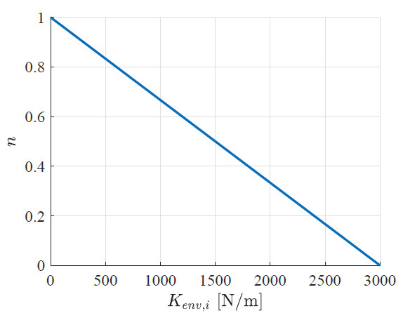
Figure 10. Adaptation law for $$ n $$ in ^[13].

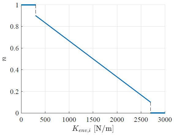
Figure 11. Proposed adaptation law for $$ n $$ in (22).

Remark 1. The environment stiffness parameter $$ K_{env, i} $$ estimation can be performed as described by the authors of ^{[21, 22]}.

Remark 2. The stability of the controller can be addressed following the work in ^{[12, 13]}.

4.1. Task description

To evaluate the performance of the improved hybrid controller, an interaction task along the vertical Cartesian direction $$ z $$ was considered. The Franka EMIKA panda robot torque controller was simulated as for the real robot, i.e., with a control frequency of $$ 1 $$ kHz. A variable stiffness environment was simulated, with an environment stiffness $$ K_{env, z} $$ varying as in Figure 12. The robot moves its setpoint down from its initial positioning of $$ 0.10 $$ m in $$ \Delta t_1=1 $$s. Then, it moves forward horizontally $$ 0.20 $$ m in $$ \Delta t_2=1 $$s, and it maintains its position for $$ \Delta t_3=3 $$s.

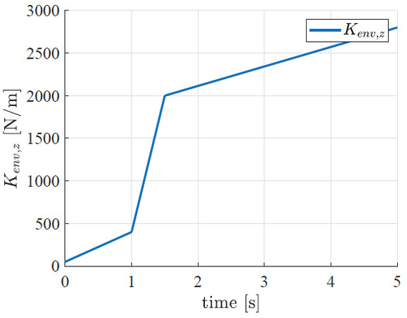
Figure 12. Variable environment stiffness $$ K_{env, z} $$ along the interaction direction $$ z $$.

4.2. Control parameters definition

The parameters for the impedance controller were chosen as follows:

The diagonal elements of the matrix $$ {\bf{D}}_d $$ were computed as follows:

The parameters of the admittance controller were imposed as follows:

where $$ K_{px}=K_{py}=K_{pz}=10000 $$ N/m and $$ K_{p \phi}=K_{p \theta}=K_{p \psi}=100 $$ Nm/rad. The diagonal elements of the matrix $$ {\bf{K}}_v $$ were defined as follows:

The values used in Equation (17) were imposed as in the following: $$ m_{0, z}=8 $$ kg, $$ \delta_{0, z}=100 $$ ms, and $$ a_z=0.68 $$. The values used for the adaptation law of $$ n_z $$ in Equation (22) were imposed as in the following: $$ K_{env, z}^{max}=2700 $$ N/m and $$ K_{env, z}^{min}=300 $$ N/m.

4.3. Results evaluation

The performance obtained when applying the hybrid control with the algebraic, differential, and iterative switching methods can be seen in Figure 13a, 13c, 13e, respectively, considering fixed and variable $$ \delta_z $$. In addition, Figure 13b, 13d, 13f shows the resulting interaction force along the Cartesian DoF $$ z $$. Figure 14 shows the applied values for the variable $$ \delta_z $$. Specifically, this figure refers to the values obtained when the algebraic switching method is applied (similar results are achieved for the other methodologies in Section 3.1). Figure 15 shows the value of $$ M_{x, zz}({\bf{q}}) $$ along the simulation upon which $$ \delta_z $$ is computed. Figure Figure 16a shows the values assumed by $$ n_z $$ when the adaptation strategy of ^[13] is used, while Figure Figure 16b shows the values obtained with the proposed adaptation strategy in Equation (22). It is possible to observe how $$ n_z $$ varies more often in the proposed adaptation strategy, assuming additional intermediate levels. When the environmental stiffness is not within the range for the medium environment (hence, within the values $$ K_{env, i}^{min} $$ and $$ K_{env, i}^{max} $$), the pure impedance or admittance controllers will be applied. This is also visible in Figure 16b, at the beginning and at the end of the simulation, where $$ n_z $$ assumes the values of $$ 1 $$ and $$ 0 $$, respectively, for a longer time in comparison to strategy proposed by Ott et al.^[13].

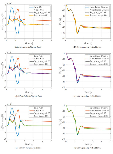
Figure 13. Hybrid control performance comparison considering fixed $$ \delta_{fix, z} $$ and $$ n_{fix, z} $$ vs. variable $$ \delta_{var, z} $$ and fixed $$ n_{fix, z} $$, together with the corresponding interaction force.

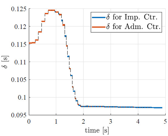
Figure 14. Variable $$ \delta_z $$ evaluated at every switch as a function of $$ M_{x, zz}(\bf{q}) $$ for the algebraic switching method.

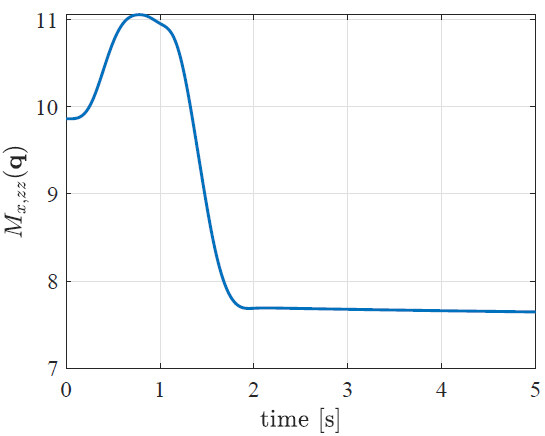
Figure 15. $$ M_{x, zz}(\bf{q}) $$ upon which $$ \delta_z $$ is evaluated.

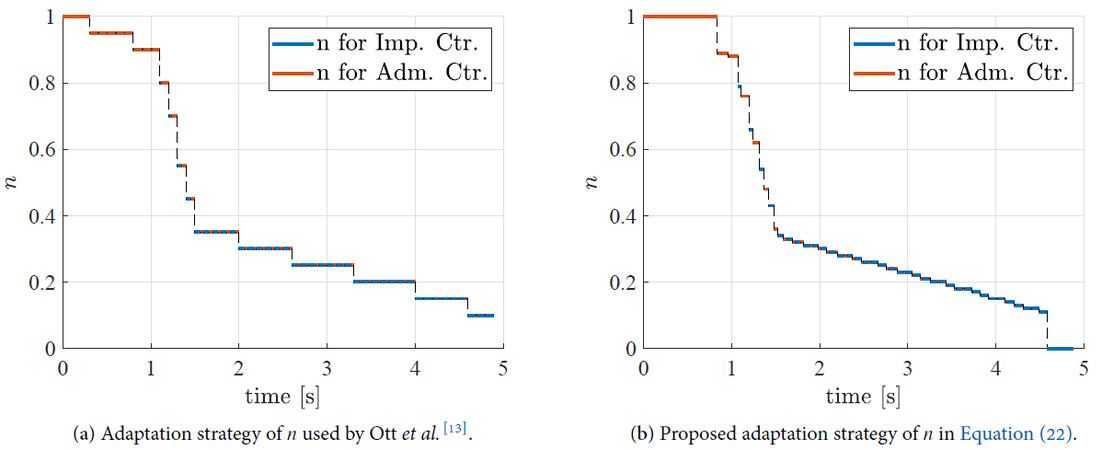
Figure 16. Comparison of the old and new adaptation strategies of $$ n $$ for the algebraic switching method.

Authors' contributions

Made substantial contributions to conception and design of the study and performed data analysis and interpretation: Roveda L, Formenti A

Performed data acquisition, as well as provided administrative, technical, and material support: Formenti A, Roveda L, Shahid AA, Piga D, Bucca G

Paper writing: Roveda L, Formenti A, Shahid AA

Supervision: Piga D, Bucca G

Availability of data and materials

Not applicable.

Financial support and sponsorship

The work has been developed within the project ASSASSINN, funded from H2020 CleanSky 2 under grant agreement n. 886977.

Conflicts of interest

All authors declared that there are no conflicts of interest.

Ethical approval and consent to participate

Not applicable.

Consent for publication

All the authors accept to publish the paper.

Copyright

© The Author(s) 2022.

REFERENCES

1. Schumacher M, Wojtusch J, Beckerle P, von Stryk O. An introductory review of active compliant control. Robotics and Autonomous Systems 2019;119:185-200.
2. Lefebvre T, Xiao J, Bruyninckx H, De Gersem G. Active compliant motion: a survey. Advanced Robotics 2005;19:479-99.
3. Calanca A, Muradore R, Fiorini P. A review of algorithms for compliant control of stiff and fixed-compliance robots. IEEE/ASME Trans Mechatron 2015;21:613-24.
4. Zhang T, Du Q, Yang G, et al. A review of compliant control for collaborative robots. In: 2021 IEEE 16th Conference on Industrial Electronics and Applications (ICIEA). IEEE; 2021. pp. 1103-8.
5. Hogan N. Impedance control: an approach to manipulation. In: 1984 American Control Conference; 1984. pp. 304-13.
6. Roveda L, Pedrocchi N, Tosatti LM. Exploiting impedance shaping approaches to overcome force overshoots in delicate interaction tasks. Int J Adv Robot Syst 2016;13:1729881416662771.
7. Roveda L, Pedrocchi N, Beschi M, Tosatti LM. High-accuracy robotized industrial assembly task control schema with force overshoots avoidance. Control Engineering Practice 2018;71:142-53.
8. Roveda L, Piga D. Robust state dependent riccati equation variable impedance control for robotic force-tracking tasks. Int J Intell Robot Appl 2020;4:507-19.
9. Hogan N. On the stability of manipulators performing contact tasks. IEEE J Robot Automat 1988;4:677-86.
10. Roveda L, Iannacci N, Vicentini F, et al. Optimal impedance force-tracking control design with impact formulation for interaction tasks. IEEE Robot Autom Lett 2016;1:130-36.
11. Schindlbeck C, Haddadin S. Unified passivity-based cartesian force/impedance control for rigid and flexible joint robots via task-energy tanks. In: 2015 IEEE international conference on robotics and automation (ICRA). IEEE; 2015. pp. 440-47.
12. Ott C, Mukherjee R, Nakamura Y. Unified impedance and admittance control. In: 2010 IEEE International Conference on Robotics and Automation; 2010. pp. 554-61.
13. Ott C, Mukherjee R, Nakamura Y. A hybrid system framework for unified impedance and admittance control. J Intell Robot Syst 2015;78:359-75.
14. Cavenago F, Voli L, Massari M. Adaptive hybrid system framework for unified impedance and admittance control. J Intell Robot Syst 2018;91:569-81.
15. Mei C, Yuan J, Guan R. Adaptive unified Impedance and Admittance control using online environment estimation. In: 2018 IEEE International Conference on Robotics and Biomimetics (ROBIO); 2018. pp. 1864-69.
16. Izadbakhsh A, Kheirkhahan P, Khorashadizadeh S. FAT-based robust adaptive control of electrically driven robots in interaction with environment. Robotica 2018;12;37:1-22.
17. Yang B, Zhai DH, Lyu W, Xia Y. Event-based hybrid impedance and admittance control. In: 2019 Chinese Control Conference (CCC); 2019. pp. 4596-601.
18. Fu L, Wu R, Zhao J. On the stability of maxwell model based impedance control and cartesian admittance control implementation. In: 2019 IEEE 4th International Conference on Advanced Robotics and Mechatronics (ICARM); 2019. pp. 793-98.
19. Siciliano B, Villani L. Robot force control. vol. 540 Springer Science & Business Media; 2012.
20. Gaz C, Cognetti M, Oliva A, Robuffo Giordano P, De Luca A. Dynamic identification of the franka emika panda robot with retrieval of feasible parameters using penalty-based optimization. IEEE Robot Autom Lett 2019;4:4147-54.
21. Roveda L, Vicentini F, Tosatti LM. Deformation-tracking impedance control in interaction with uncertain environments. In: 2013 IEEE/RSJ International Conference on Intelligent Robots and Systems; 2013. pp. 1992-97.
22. Roveda L, Shahid AA, Iannacci N, Piga D. Sensorless optimal interaction control exploiting environment stiffness estimation. IEEE Trans Contr Syst Technol 2022;30:218-33.
23. Xu Z, Li S, Zhou X, Zhou S, et al. Dynamic neural networks for motion-force control of redundant manipulators: an optimization perspective. IEEE Trans Ind Electron 2021;68:1525-36.
Cite This Article
Export citation file: BibTeX | RIS
OAE Style
Formenti A, Bucca G, Shahid AA, Piga D, Roveda L. Improved impedance/admittance switching controller for the interaction with a variable stiffness environment. Complex Eng Syst 2022;2:12. http://dx.doi.org/10.20517/ces.2022.16
AMA Style
Formenti A, Bucca G, Shahid AA, Piga D, Roveda L. Improved impedance/admittance switching controller for the interaction with a variable stiffness environment. Complex Engineering Systems. 2022; 2(3): 12. http://dx.doi.org/10.20517/ces.2022.16
Chicago/Turabian Style
Formenti, Alessandro, Giuseppe Bucca, Asad Ali Shahid, Dario Piga, Loris Roveda. 2022. "Improved impedance/admittance switching controller for the interaction with a variable stiffness environment" Complex Engineering Systems. 2, no.3: 12. http://dx.doi.org/10.20517/ces.2022.16
ACS Style
Formenti, A.; Bucca G.; Shahid AA.; Piga D.; Roveda L. Improved impedance/admittance switching controller for the interaction with a variable stiffness environment. Complex. Eng. Syst. 2022, 2, 12. http://dx.doi.org/10.20517/ces.2022.16
About This Article
Copyright
Data & Comments
Data
Cite This Article 26 clicks
Like This Article 49
likes
Comments
Comments must be written in English. Spam, offensive content, impersonation, and private information will not be permitted. If any comment is reported and identified as inappropriate content by OAE staff, the comment will be removed without notice. If you have any queries or need any help, please contact us at support@oaepublish.com.